MiniGPT in JAX: 3D Parallelism for Scalable Transformer Training

Part 1: Single node — Multi GPU

Part 2: Multi node with Jax & Ray

The idea of hardware-agnostic deep learning frameworks has long been an appealing abstraction, especially in early PyTorch designs, where it often felt as though models could be written independently of the underlying hardware. In practice, however, achieving efficient large-scale training inevitably requires explicit consideration of device placement, memory movement, and inter-device communication through collectives. Once performance and scale become critical, developers are inevitably drawn into the details of kernel optimization and synchronization across devices.

As a result, a range of frameworks and ecosystem efforts have emerged to bridge this gap between abstraction and performance. In the PyTorch ecosystem, efforts such as graph-level compilation and kernel optimization in PyTorch Inductor, low-level kernel programming via Triton, and large-scale distributed training systems like Megatron-LM represent different points in the design space between usability and control. Under the hood, these systems rely heavily on communication primitives such as NCCL for GPUs, GLOO for CPUs, and XLA-coordinated collectives on TPUs, all of which implement the core idea of efficient multi-device synchronization.

At the center of this design space is the Single Program Multiple Data (SPMD) paradigm, where developers ideally write a single forward and backward computation, while the framework automatically injects the necessary communication and partitioning logic to execute it across multiple devices. This creates a fundamental trade-off between implicitness and ease of use versus explicit control and expressiveness.

In this context, JAX represents a particularly strong approach to structured parallelism, offering a compiler-driven abstraction for expressing data, model, and pipeline parallelism in a unified way. In this article, we use MiniGPT as a running example to demonstrate how different parallelism strategies can be implemented in JAX and compare them with familiar PyTorch-based approaches. The discussion is inspired by the mini-course Build and Train an LLM with JAX from DeepLearning.AI.

MINIGPT

We first start with the definition of MiniGPT network. It has a TokenAndPositionEmbedding layer followed by several TransformerBlocks; each with MHA(Multi-head attention) and finally a linear projection output layer:

Mini-GPT network architecture

class TransformerBlock(nnx.Module):

    def __init__(self, embed_dim, num_heads, ff_dim, *, rngs):

        self.attention = nnx.MultiHeadAttention(
            num_heads=num_heads,
            in_features=embed_dim,
            qkv_features=embed_dim,
            out_features=embed_dim,
            decode=False,
            rngs=rngs
        )

    def __call__(self, x, mask=None):
        attn_out = self.attention(x, mask=mask)
        x = x + attn_out
        return x

class TokenAndPositionEmbedding(nnx.Module):
    def __init__(self, maxlen, vocab_size, embed_dim, *, rngs):
        self.token_emb = nnx.Embed(vocab_size, embed_dim, rngs=rngs)
        self.pos_emb = nnx.Embed(maxlen, embed_dim, rngs=rngs)

    def __call__(self, x):
        seq_len = x.shape[1]
        positions = jnp.arange(seq_len)[None, :]
        return self.token_emb(x) + self.pos_emb(positions)

class MiniGPT(nnx.Module):

    def __init__(self, maxlen=maxlen, vocab_size=vocab_size, embed_dim=embed_dim, num_heads=num_heads,
                 feed_forward_dim=feed_forward_dim, num_transformer_blocks=num_transformer_blocks, *, rngs=nnx.Rngs(0)):

        self.maxlen = maxlen

        self.embedding = TokenAndPositionEmbedding(maxlen, vocab_size, embed_dim, rngs=rngs)

        self.transformer_blocks = [
            TransformerBlock(embed_dim, num_heads, feed_forward_dim, rngs=rngs)
            for _ in range(num_transformer_blocks)
        ]

        self.output_layer = nnx.Linear(embed_dim, vocab_size, use_bias=False, rngs=rngs)

    def causal_attention_mask(self, seq_len):
        return jnp.tril(jnp.ones((seq_len, seq_len)))

    def __call__(self, token_ids):
        seq_len = token_ids.shape[1]
        mask = self.causal_attention_mask(seq_len)

        x = self.embedding(token_ids)

        for block in self.transformer_blocks:
            x = block(x, mask=mask)

        logits = self.output_layer(x)

        return logits

DATA PARALLEL

Data parallelism in JAX follows the same core idea as PyTorch’s DP: the input batch is partitioned across devices while model parameters are replicated. This is typically expressed through a device mesh and a sharding specification:

mesh = Mesh(mesh_utils.create_device_mesh((8,)), ('batch',))
batch_to_pass = jax.device_put(
    (input_batch, target_batch), NamedSharding(mesh, P("batch", None))
)

Assuming 8 GPUs, the 1D device mesh defines a single axis 'batch', meaning all devices participate in splitting the batch dimension. The partition specification P('batch', None) instructs JAX to shard the first dimension of the input tensor (the batch dimension) across the 8 devices, while keeping the remaining dimensions (e.g., sequence length) fully replicated. As a result, an input of shape (B,T) is partitioned into 8 local shards of shape (B/8,T), each residing on a different device.

The same model’s ‘params’ are replicated across devices and this forward function is executed in an SPMD fashion:

loss = model(batch_to_pass, params)

This is equivalent to conceptual SPMD execution:

for device in devices:
    loss_i = model(local_batch_i, replicated_params)

In JAX, the combination of jit compilation and jax.value_and_grad enables fully compiled reverse-mode automatic differentiation. The JIT compiler traces both the forward computation and its corresponding backward pass into a single functional program. As a result, both forward and backward passes are fused and compiled into a single optimized executable that runs efficiently on hardware accelerators, minimizing Python overhead and enabling cross-device optimization of the entire training step.

@nnx.jit
def train_step(model, optimizer, metrics, batch):
    grad_fn = nnx.value_and_grad(loss_fn, has_aux=True)
    (loss, logits), grads = grad_fn(model, batch)
    metrics.update(loss=loss, logits=logits, labels=batch[1])
    optimizer.update(grads)

During both forward and backward passes, each device independently computes activations and gradients on its local batch shard. Gradient synchronization is then performed across the 'batch' axis using an all-reduce, ensuring that parameter updates remain consistent across all data-parallel replicas. This behavior is efficiently orchestrated by nnx.jit, which compiles the full step function into an optimized SPMD program and transparently inserts the necessary collective communication across devices.

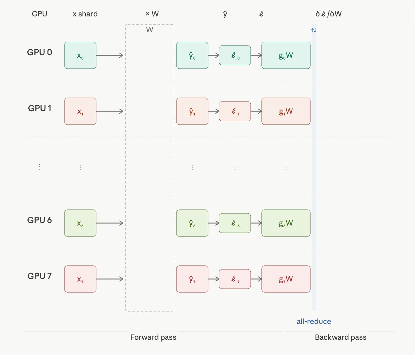
Simplified to a single shared weight W. Each GPU now goes directly x_i → (×W) → ŷ_i → ℓ_i → ∂ℓ/∂W, with a single all-reduce column syncing the gradients across all 8 devices.

In earlier JAX-style APIs based on pmap, synchronization had to be expressed explicitly in the user code. The programmer manually specified the data-parallel axis and inserted collective operations such as jax.lax.pmean to ensure consistency across devices:

import functools

# Remember that the 'batch' is just an arbitrary string label used
# to later tell 'jax.lax.pmean' which axis to reduce over. Here, we call it
# 'batch', but could have used anything, so long as 'pmean' used the same.
@functools.partial(jax.pmap, axis_name='batch')
def update(params: Params, x: ArrayLike, y: ArrayLike) -> Any:
    # Compute the gradients on the given minibatch (individually on each device)
    loss, grads = jax.value_and_grad(loss_fn)(params, x, y)

    # Combine the gradient across all devices (by taking their mean)
    grads = jax.lax.pmean(grads, axis_name='batch')

    # Also combine the loss. Unnecessary for the update, but useful for logging
    loss = jax.lax.pmean(loss, axis_name='batch')

    # Each device performs its own update, but since we start with the same params
    # and synchronise gradients, the params stay in sync
    LEARNING_RATE = 1e-3
    new_params = jax.tree_map(
       lambda param, g: param - g * LEARNING_RATE, params, grads)
    return new_params, loss

In the modern JAX programming model, this manual orchestration is largely removed. With jit compilation, device meshes, and NamedSharding, the compiler infers the distributed execution strategy and automatically inserts the required collectives. In particular, gradient synchronization across the data-parallel axis is lowered into an all-reduce equivalent of pmean, without requiring explicit user annotations. This allows the entire update step to be expressed as a single function, while the compiler handles partitioning and communication transparently.

TENSOR PARALLEL

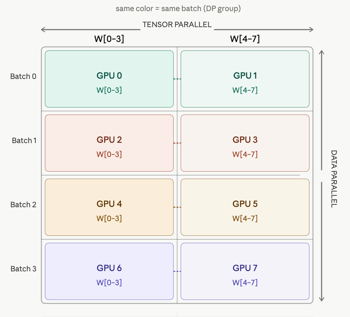
You can shard a tensor either column-wise or row-wise. Consider two consecutive linear layers without bias, W1​ and W2, applied as x@W1@W2​. In a tensor-parallel (TP) setup, one option is to apply a column-wise partitioning to W1​ followed by a row-wise partitioning to W2. This corresponds to the standard Megatron-style transformer pattern, where the intermediate activations are kept partially after the column-wise projection and then all-reduced after the row-wise projection to aggregate partial outputs across tensor-parallel ranks.

As an alternative, consider a single linear layer (without bias) using only a column-wise split under the same TP × DP configuration. Here, the forward pass requires an all-gather across TP ranks to assemble the full output activation, while gradients during backpropagation are typically handled via all-reduce to accumulate contributions across shards.

In both cases, assume a total of 8 devices organized into 4 data-parallel (DP) groups, each containing 2 tensor-parallel (TP) workers.

Within each DP group (a pair of GPUs), the behavior differs as follows:

• Example 1 (two-layer model: x@W1@W2​): W1​ is column-sharded across TP ranks(2), producing partial activations. These activations are then passed into W2, which is row-sharded; its outputs are combined using an all-reduce across TP ranks to produce the final result per DP group. DP synchronization (typically all-reduce) then aggregates gradients across the 4 DP groups.

TP Example 1: Inside a DP group for 2 linear layers with collective — ‘all-reduce’

• Example 2 (single linear layer, column-sharded W): Each TP rank computes a partial output from its shard of W. An all-gather across the 2 TP workers within the DP group reconstructs the full activation. During backpropagation, gradients are aggregated using all-reduce across TP ranks, followed by DP-level synchronization across the 4 groups. Note that, typically in a column-parallel linear layer, outputs are usually kept partitioned, and an all-gather across TP ranks within each DP group is only used if a full activation is required (e.g., at the end of a TP block). Otherwise, the next layer is typically row-parallel, avoiding reconstruction and using an all-reduce instead of all-gather for efficiency like shown in Example 1. In backpropagation, gradients w.r.t. inputs are all-reduced across TP ranks, weight gradients stay local, and final synchronization is performed via DP all-reduce across the 4 groups.

TP Example 2: Inside a DP group of 1 Linear layer with collective ‘all-gather’

Manual ‘pmap’ style for 1 Linear layer ‘x@W’ example looks like this:

# Shard parameters
def shard_params(params, tp_size, dp_size):
    # Split layer weights by tp_size, then replicate for dp_size
    # Example for a linear layer [in, out] -> [in, out/tp_size]
    return jax.tree_map(lambda x: x.reshape(dp_size, tp_size, -1), params)

# Example Parallel Layer
def parallel_linear(x, weight_shard):
    # x is (batch/dp_size, hidden)
    # weight_shard is (hidden, hidden/tp_size)
    return jnp.matmul(x, weight_shard)

# Pmap over all devices (DP * TP)
@partial(pmap, axis_name='device_axis')
def forward(params, batch):
    # 1. Local MatMul
    hidden = parallel_linear(batch, params['layer1'])
    # 2. Sync TP devices (All-Gather to reunite hidden states)
    hidden = lax.all_gather(hidden, axis_name='device_axis') # Simplified
    return hidden

Luckily you don’t have to do that anymore with Jax’s JIT, instead just define a 2D mesh with TP and DP as dimension and give each tensor/layer operation a hint of how they should be sharded:

mesh = Mesh(mesh_utils.create_device_mesh((4, 2)), ('batch', 'model'))

class TransformerBlock(nnx.Module):
    """ A single Transformer block.

    Each Transformer block processes input sequences via self-attention and feed-forward networks.

    Args:
        embed_dim (int): Embedding dimensionality.
        num_heads (int): Number of attention heads.
        ff_dim (int): Dimensionality of the feed-forward network.
        rngs (flax.nnx.Rngs): A Flax NNX stream of JAX PRNG keys.
        rate (float): Dropout rate. Defaults to 0.1.
    """
    def __init__(
        self,
        embed_dim: int,
        num_heads: int,
        ff_dim: int,
        *,
        rngs: nnx.Rngs,
        mesh: Mesh,
        rate: float = 0.1,
    ):
        # Multi-Head Attention (MHA) with `flax.nnx.MultiHeadAttention`.
        # Specifies tensor sharding (depending on the mesh configuration)
        # where we shard the weights across devices for parallel computation.
        self.mha = nnx.MultiHeadAttention(
            num_heads=num_heads,
            in_features=embed_dim,
            kernel_init=nnx.with_partitioning(
                nnx.initializers.xavier_uniform(),
                NamedSharding(mesh, P(None, 'model'))
            ),
            bias_init=nnx.with_partitioning(
                nnx.initializers.zeros_init(),
                NamedSharding(mesh, P('model'))
            ),
            rngs=rngs
        )
        # The first dropout with `flax.nnx.Dropout`.
        self.dropout1 = nnx.Dropout(rate=rate)
        # First layer normalization with `flax.nnx.LayerNorm`.
        self.layer_norm1 = nnx.LayerNorm(
            epsilon=1e-6,
            num_features=embed_dim,
            scale_init=nnx.with_partitioning(
                nnx.initializers.ones_init(),
                NamedSharding(mesh, P('model'))
            ),
            bias_init=nnx.with_partitioning(
                nnx.initializers.zeros_init(),
                NamedSharding(mesh, P('model'))
            ),
            rngs=rngs
        )
        # The first linear transformation for the feed-forward network with `flax.nnx.Linear`.
        self.linear1 = nnx.Linear(
            in_features=embed_dim,
            out_features=ff_dim,
            kernel_init=nnx.with_partitioning(
                nnx.initializers.xavier_uniform(),
                NamedSharding(mesh, P(None, 'model'))
            ),
            bias_init=nnx.with_partitioning(
                nnx.initializers.zeros_init(),
                NamedSharding(mesh, P('model'))
            ),
            rngs=rngs
        )
        # The second linear transformation for the feed-forward network with `flax.nnx.Linear`.
        self.linear2 = nnx.Linear(
            in_features=ff_dim,
            out_features=embed_dim,
            kernel_init=nnx.with_partitioning(
                nnx.initializers.xavier_uniform(),
                NamedSharding(mesh, P(None, 'model'))
            ),
            bias_init=nnx.with_partitioning(
                nnx.initializers.zeros_init(),
                NamedSharding(mesh, P('model'))
            ),
            rngs=rngs
        )
        # The second dropout with `flax.nnx.Dropout`.
        self.dropout2 = nnx.Dropout(rate=rate)
        # Second layer normalization with `flax.nnx.LayerNorm`.
        self.layer_norm2 = nnx.LayerNorm(
            epsilon=1e-6,
            num_features=embed_dim,
            scale_init=nnx.with_partitioning(
                nnx.initializers.ones_init(),
                NamedSharding(mesh, P(None, 'model'))
            ),
            bias_init=nnx.with_partitioning(
                nnx.initializers.zeros_init(),
                NamedSharding(mesh, P(None, 'model'))
            ),
            rngs=rngs
        )

    # Apply the Transformer block to the input sequence.
    def __call__(self, inputs, training: bool = False):
        input_shape = inputs.shape
        _, seq_len, _ = input_shape

        # Instantiate the causal attention mask.
        mask = causal_attention_mask(seq_len)

        # Apply Multi-Head Attention with the causal attention mask.
        attention_output = self.mha(
            inputs_q=inputs,
            mask=mask,
            decode=False
        )
        # Apply the first dropout.
        attention_output = self.dropout1(attention_output, deterministic=not training)
        # Apply the first layer normalization.
        out1 = self.layer_norm1(inputs + attention_output)

        # The feed-forward network.
        # Apply the first linear transformation.
        ffn_output = self.linear1(out1)
        # Apply the ReLU activation with `flax.nnx.relu`.
        ffn_output = nnx.relu(ffn_output)
        # Apply the second linear transformation.
        ffn_output = self.linear2(ffn_output)
        # Apply the second dropout.
        ffn_output = self.dropout2(ffn_output, deterministic=not training)
        # Apply the second layer normalization and return the output of the Transformer block.
        return self.layer_norm2(out1 + ffn_output)

class MiniGPT(nnx.Module):
    """ A miniGPT transformer model, inherits from `flax.nnx.Module`.

    Args:
        maxlen (int): Maximum sequence length.
        vocab_size (int): Vocabulary size.
        embed_dim (int): Embedding dimensionality.
        num_heads (int): Number of attention heads.
        feed_forward_dim (int): Dimensionality of the feed-forward network.
        num_transformer_blocks (int): Number of transformer blocks. Each block contains attention and feed-forward networks.
        rngs (nnx.Rngs): A Flax NNX stream of JAX PRNG keys.
    """
    # Initialize miniGPT model components.
    def __init__(
        self,
        maxlen: int, 
        vocab_size: int, 
        embed_dim: int, 
        num_heads: int, 
        feed_forward_dim: int, 
        num_transformer_blocks: int, 
        rngs: nnx.Rngs,
        mesh: Mesh,
    ):
        # Initiliaze the `TokenAndPositionEmbedding` that combines token and positional embeddings.
        self.embedding_layer = TokenAndPositionEmbedding(
            maxlen, vocab_size, embed_dim, rngs=rngs
        )
        # Create a list of `TransformerBlock` instances.
        # Each block processes input sequences using attention and feed-forward networks.
        self.transformer_blocks = [
            TransformerBlock(
                embed_dim=embed_dim, 
                num_heads=num_heads, 
                ff_dim=feed_forward_dim,
                rngs=rngs,
                mesh=mesh,
            ) for _ in range(num_transformer_blocks)
        ]
        # Initialize the output `flax.nnx.Linear` layer producing logits over the vocabulary for next-token prediction.
        self.output_layer = nnx.Linear(
            in_features=embed_dim,
            out_features=vocab_size,
            kernel_init=nnx.with_partitioning(
                nnx.initializers.xavier_uniform(), 
                NamedSharding(mesh, P(None, 'model'))
            ),
            bias_init=nnx.with_partitioning(
                nnx.initializers.zeros_init(), 
                NamedSharding(mesh, P(None, 'model'))
            ),
            rngs=rngs
        )

    def __call__(self, inputs, training: bool = False):
        # Pass the input tokens through the `embedding_layer` to get token embeddings.
        # Apply each transformer block sequentially to the embedded input, use the `training` flag for the behavior of `flax.nnx.Dropout`.
        x = self.embedding_layer(inputs)
        for transformer_block in self.transformer_blocks:
            x = transformer_block(x, training=training)
        # Pass the output of the transformer blocks through the output layer,
        # and obtain logits for each token in the vocabulary (for next token prediction).
        outputs = self.output_layer(x)
        return outputs

Now take a closer look at the sharding hint ‘NamedSharding’ at each individual layer:

kernel_init=nnx.with_partitioning(
    nnx.initializers.xavier_uniform(), 
    NamedSharding(mesh, P(None, 'model'))
)

basically means sharding the kernel weight ‘W’ along its second dimension (column-wise) and allocate the sharded parameters W_i’s along ‘model’ dimension of the given device mesh ‘mesh’.

Similarly this line in MHA’s linear layer 1:

bias_init=nnx.with_partitioning(
    nnx.initializers.zeros_init(),
    NamedSharding(mesh, P('model'))
)

means to initialise the bias of dimension (h1,) and split h1 across the model axis of the mesh.

Note that the NamedSharding follows strictly the dimension of the tensor to tell exactly how sharding across its different dimension(s) is to be done. Once these sharding annotations are present, XLA can reason about communication automatically. Because every parameter and intermediate activation carries a layout contract, XLA can:

• Infer when tensor shapes are partially distributed
• Detect mismatches between local shards and required global views
• Insert the appropriate collective operations such as all-gather (to reconstruct full tensors from distributed shards), all-reduce (to aggregate gradients across devices), and all-to-all / all-permute (to exchange or rearrange data between devices according to a specified permutation pattern).

The remaining step is to place the input tensor (of shape B×Seq) onto the defined 2D device mesh, sharding it along its first dimension:

for epoch in range(num_epochs):
    for batch in text_dl:
        if len(batch) % len(jax.devices()) != 0:
            continue  # skip the remaining elements
        input_batch = jnp.array(jnp.array(batch).T)
        target_batch = prep_target_batch(input_batch)
        batch_to_pass = jax.device_put(
            (input_batch, target_batch), NamedSharding(mesh, P("batch", None))
        )
        train_step(
            model,
            optimizer,
            metrics,
            batch_to_pass,
            num_stages,
        )

So now you can start to see how XLA is able to determine which collective operations to insert in a full tensor-parallel program based on the device mesh layout and the NamedSharding specifications.

MiniGPT dataflow for 2D mesh (batch=M,model=T) with TP+DP

PIPELINE PARALLEL

So instead of splitting the model horizontally each tensor by column or row, we can also split by layers for example: split the 8 transformer blocks into 2 stages:

Stage 0: block0->3

Stage 1: block4->7

We can do a mixture of PP, TP and DP by defining a 3D mesh of stage, batch and model dimensions:

mesh = Mesh(mesh_utils.create_device_mesh((2, 2, 2)), ('stage', 'batch', 'model'))

3D mesh across 8 devices

Even stage 1 depends on stage 0, the forward pass (and subsequently backward pass) however executes on different micro-batches A & B, therefore there is some overlapping on which GPipe style execution can be useful:

Forward overlap in timeline of GPipe

In the older pmap-based GPipe-style pipeline, computation is split into G stages and executed with manual micro-batch scheduling. Each stage runs on a separate device, and activations are passed through a shifting pipeline buffer using jax.pmap. Micro-batches are streamed to overlap computation across stages, and outputs are collected from the final stage after a warm-up of G−1 steps once the pipeline is filled.

# stack weights according to stages
params = stack_stage_weights(params)
# create shifting buffer
state = jnp.zeros((G, micro_batch_size, d))
y_pred = []
for i in range(M + G - 1):
    from_prev_stage = jnp.concatenate([jnp.expand_dims(x[i], 0), state[:-1]])
    state = jax.pmap(model)(from_prev_stage, params)
    if i >= G - 1: # first micro-batch has passed through the last stage
        y_pred.append(state[-1])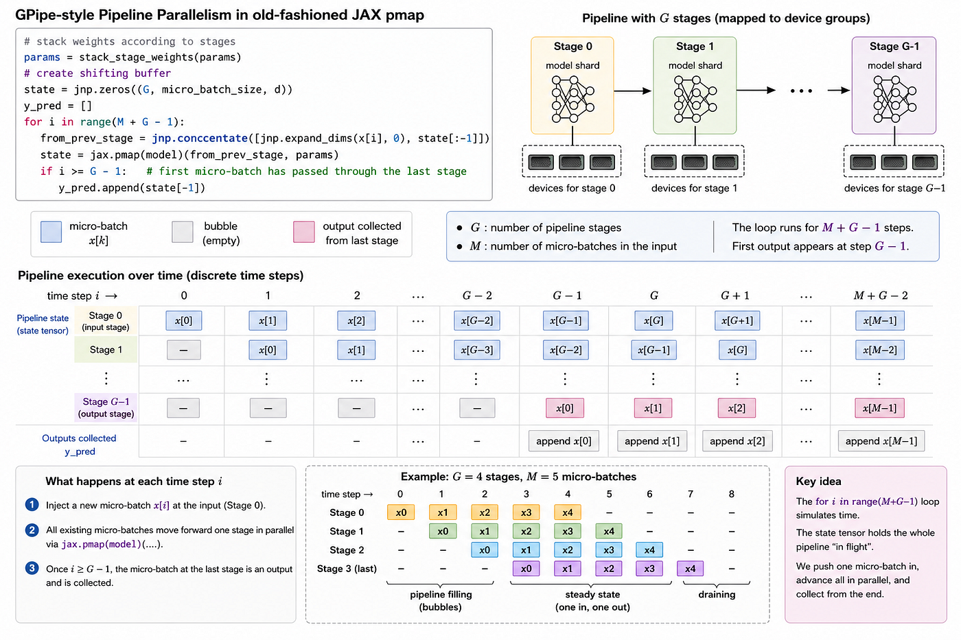

GPipeline with micro-batches

You can observe that micro-batches are explicitly scheduled and overlapped across pipeline stages to maximize device utilization and reduce idle time. In contrast, modern JIT-based implementations remove this manual orchestration by relying on compiler-driven scheduling, which automatically constructs an optimized execution plan that manages micro-batch interleaving and pipeline parallelism transparently.

def split_stages(blocks, num_stages):
    L = len(blocks)
    assert L % num_stages == 0

    stage_size = L // num_stages
    return [
        blocks[i * stage_size:(i + 1) * stage_size]
        for i in range(num_stages)
    ]

def run_stage(blocks, x, training):
    for block in blocks:
        x = block(x, training=training)
    return x

def get_stage_mesh(mesh, stage_id):
    # mesh.devices: (stage, batch, model)
    stage_devices = mesh.devices[stage_id, :, :]

    return Mesh(
        stage_devices,
        ('batch', 'model')
    )

def make_stage_fn(blocks, stage_id, mesh):

    stage_mesh = get_stage_mesh(mesh, stage_id)

    stage_sharding = NamedSharding(stage_mesh, P('batch','model'))

    @partial(jax.jit, static_argnames=['training'])
    def stage_fn(x, training=False):
        x = jax.lax.with_sharding_constraint(x, stage_sharding)
        x = run_stage(blocks, x, training)
        return x

    return stage_fn

class PipelineMiniGPT(nnx.Module):

    def __init__(self, base_model: MiniGPT, num_stages: int):
        self.base_model = base_model
        self.embed = base_model.embedding_layer
        self.output = base_model.output_layer

        self.blocks = split_stages(
            base_model.transformer_blocks,
            num_stages
        )

        self.num_stages = num_stages
        self.mesh = get_mesh(mode='PPTPDP')

        # compile each stage
        self.stage_fns = [
            make_stage_fn(stage, i, self.mesh)
            for i, stage in enumerate(self.blocks)
        ]

    def forward(self, x, training=False):

        # embedding (replicated or sharded over batch)
        x = self.embed(x)

        # pipeline stages
        for fn in self.stage_fns:
            x = fn(x, training)

        # output projection
        x = self.output(x)

        return x

In this design, XLA does not explicitly “schedule a pipeline” in the way GPipe does with a manual micro-batch loop. Instead, the pipeline behavior emerges from the combination of jit, pjit/pmap, and mesh-based sharding, which together compile the computation into a distributed dataflow graph. Temporal dependencies between stages (e.g., stage 0 → stage 1) are transformed into spatial execution across different device partitions in the mesh.

When the model is JIT-compiled (e.g., via an nnx.Module or functional JAX transform), each stage function is traced and lowered independently. A wrapper such as make_stage_fn(stage, i, mesh) typically wraps each stage into a jax.jit-compiled SPMD unit, constrained to execute only on its assigned device slice (e.g., devices 0–3 for stage 0, devices 4–7 for stage 1). As a result, each stage becomes an isolated executable region bound to a specific mesh partition.

From XLA’s perspective, each stage is not Python code but a separately compiled computation shard in the global program, with communication between stages expressed purely through explicit sharded tensors and collectives in the compiled graph.

def get_stage_mesh(mesh, stage_id):
    # mesh.devices: (stage, batch, model)
    stage_devices = mesh.devices[stage_id, :, :]

    return Mesh(
        stage_devices,
        ('batch', 'model')
    )

def make_stage_fn(blocks, stage_id, mesh):

    stage_mesh = get_stage_mesh(mesh, stage_id)

    stage_sharding = NamedSharding(stage_mesh, P('batch','model'))

    @partial(jax.jit, static_argnames=['training'])
    def stage_fn(x, training=False):
        x = jax.lax.with_sharding_constraint(x, stage_sharding)
        x = run_stage(blocks, x, training)
        return x

    return stage_fn

jax.lax.with_sharding_constraint is a GSPMD primitive that lets you override XLA’s automatic sharding decisions by explicitly enforcing a desired partitioning on intermediate tensors inside a jit-compiled function. It is analogous to jax.device_put, which controls input placement, but operates on intermediate activations, giving fine-grained control over how data is partitioned across the device mesh during execution.

batch_to_pass = jax.device_put(
    (input_batch, target_batch), NamedSharding(mesh, P("batch", None))
)

Two independent SPMD programs (stages), each running DP×TP internally, connected by compiler-managed dataflow across device groups. Execution looks like this:

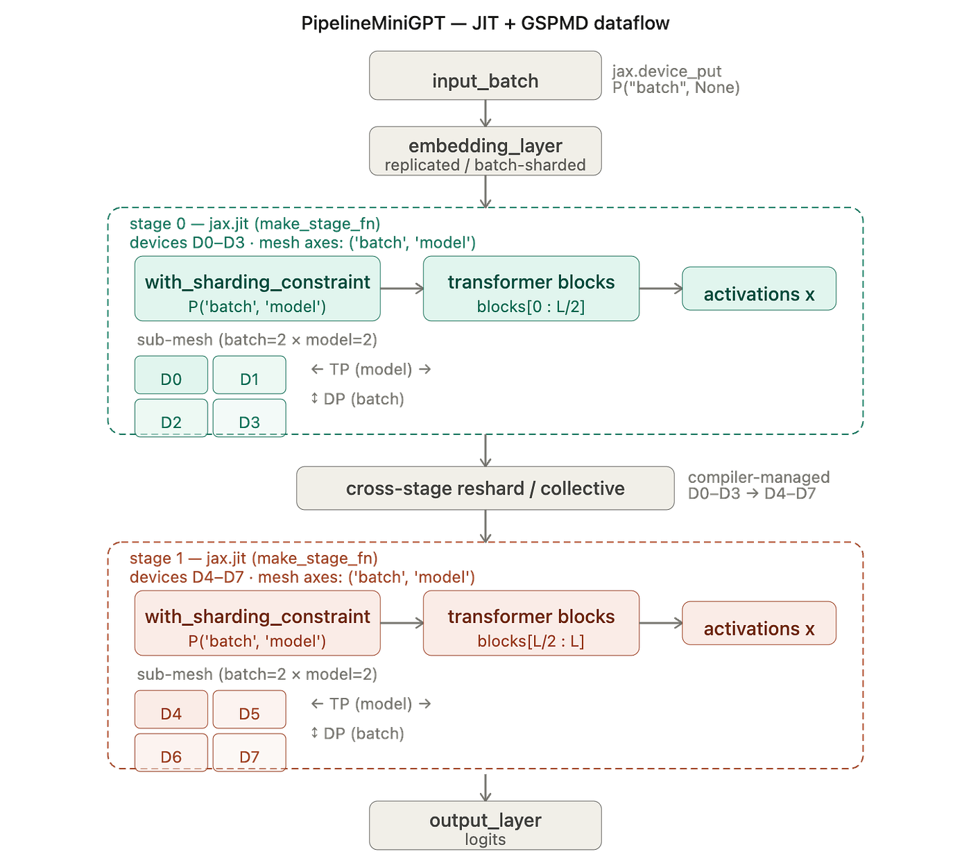
PipelineMiniGPT dataflow for 3D mesh (stage=2,batch=2,model=2) with PP+TP+DP

PYTORCH IMPLEMENTATION

In a PyTorch-based implementation of MiniGPT-style models, distributed training is typically assembled in a more manual and orchestration-heavy manner compared to JAX-based systems. Data parallelism (DP) is relatively straightforward thanks to built-in primitives like DistributedDataParallel (DDP) and legacy DataParallel, which handle gradient synchronization automatically across replicas. However, extending this to tensor parallelism (TP) and pipeline parallelism (PP) becomes significantly more complex, as PyTorch does not natively provide a unified abstraction for multi-dimensional parallelism.

As a result, TP and PP are usually implemented through custom frameworks that explicitly manage tensor partitioning, device placement, and inter-device communication. This involves manually splitting weights and activations across GPUs, coordinating collectives such as all-reduce and all-gather, and carefully orchestrating forward and backward data flows across pipeline stages. For example, research frameworks like QuintNet implement this by wrapping model components and explicitly controlling tensor sharding and cross-device execution in a fine-grained way.

In contrast, JAX-based implementations (e.g., using pjit and XLA-compiled shard_map) treat parallelism more declaratively. Instead of manually coordinating communication, the compiler infers sharding strategies from annotated mesh specifications and automatically lowers them into optimized collectives. This makes TP + PP composition significantly cleaner in JAX, where MiniGPT-like models can be expressed as a single staged computation with compiler-managed partitioning, rather than a collection of manually synchronized device programs.

Full python code: https://github.com/JustinDuy/mini-gpt

References:

https://docs.jaxstack.ai/en/latest/JAX_for_LLM_pretraining.html

[embed]GitHub - Wodlfvllf/QuintNet: QuintNet is a research-oriented PyTorch framework designed to explore… QuintNet is a research-oriented PyTorch framework designed to explore and implement multi-dimensional parallelism…github.com

https://astralord.github.io/posts/exploring-parallel-strategies-with-jax/