Distributed Systems in Machine Learning, and foundations to frontier practice

A systems-level view of distributed training: parallelism, communication, and constraints

Let’s start with the question that makes this whole field exist: why can’t you just train on one GPU?

Two walls hit you as models grow.

The compute wall. Training is dominated by matrix multiplications, and the number of floating-point operations scales with both model size and dataset size. A single GPU has a fixed FLOPs/second ceiling. Past a certain model size, one GPU would take years to finish a run that needs to finish in weeks.

The memory wall: this one bites earlier and harder. To train a model with N parameters using Adam, you need roughly: the weights themselves (2 bytes/param in bf16), gradients (2 bytes/param), and Adam’s optimizer states, momentum and variance, typically kept in fp32 for stability (8 bytes/param). That’s already ~12–16 bytes per parameter before you’ve stored a single activation. A 70-billion-parameter model needs on the order of a terabyte just for weights + gradients + optimizer state. No single GPU (even one with 80–140GB of memory) holds that.

So distributed training isn’t an optimization, it’s a requirement. Every design in this space answers one of two independent questions:

1. What do we split : the data the model sees, or the model itself?
2. How do the split-up workers get back in sync : and at what communication cost?

Let’s build both up from scratch.

Splitting the data: data parallelism

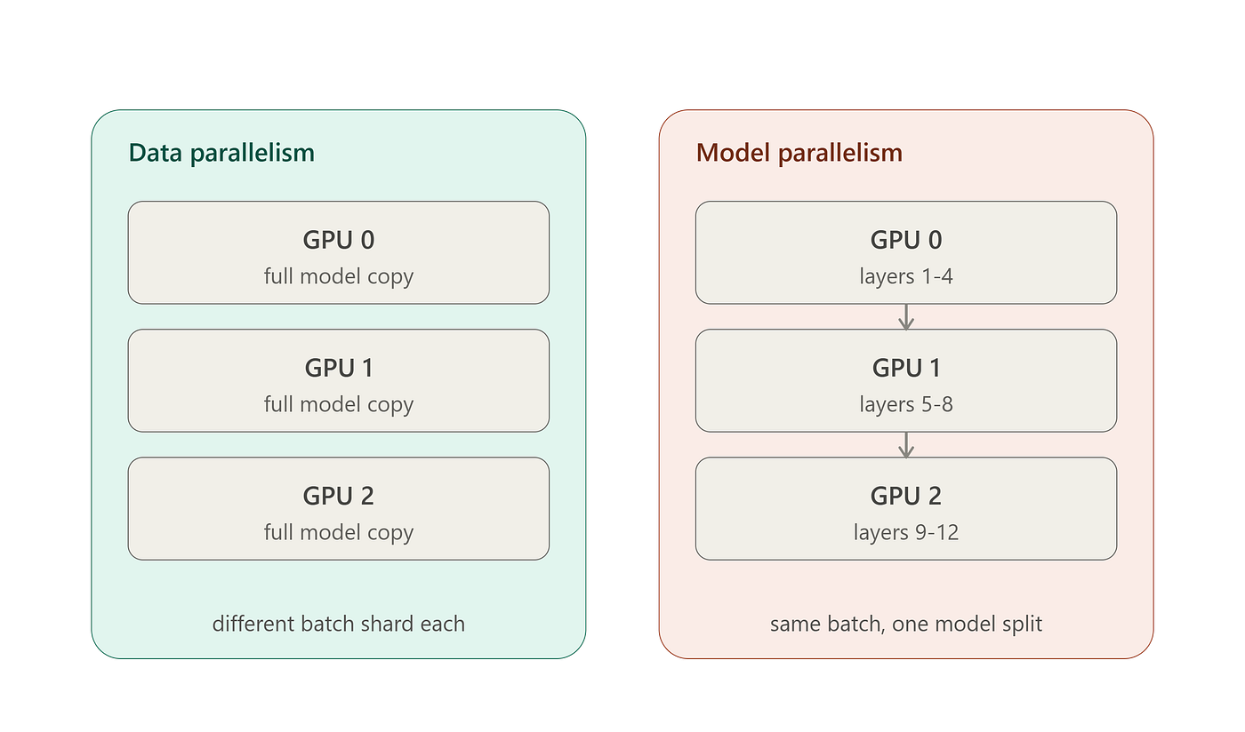
This is the simplest and most common strategy, so build the intuition here first. Give every GPU a full copy of the model. Split your batch into shards, one per GPU. Each GPU runs forward and backward on its own shard, completely independently, no communication needed during the forward/backward pass itself.

The catch: each GPU now has different gradients, computed from different data. Before you update the weights, every replica needs to end up with the same averaged gradient , otherwise your model copies drift apart and you no longer have one model, you have N slightly different ones. That averaging step is where communication enters, and it’s the single most important primitive in this entire field.

Splitting the model: model parallelism

When the model itself doesn’t fit in one GPU’s memory, you have to cut the model, not the data. There are two genuinely different ways to cut it, and mixing them up is the most common freshman confusion:

Tensor parallelism cuts within a layer. A big matrix multiply gets split, half the columns of a weight matrix live on GPU 0, half on GPU 1. Both GPUs compute their partial result, and now the partial results need to be combined before the next layer can proceed. This means communication happens inside every single layer’s forward and backward pass, extremely frequent, so it demands very fast interconnects (more on this below).

Pipeline parallelism cuts across layers. GPU 0 holds layers 1–8, GPU 1 holds layers 9–16, and so on. Data flows through like an assembly line. Communication only happens at the boundary between stages, far less frequent than tensor parallelism, so it tolerates slower links between machines.

Here’s the split visualized:

The primitive everything depends on: AllReduce

Back to data parallelism’s loose end: how do N GPUs, each holding a different gradient, end up with the same averaged gradient efficiently?

The naive approach is a parameter server: one designated machine receives every GPU’s gradients, averages them, and broadcasts the result back. This works, but that one server becomes a bandwidth bottleneck, its incoming and outgoing traffic scales with the number of workers.

The elegant fix, and one of the genuinely beautiful ideas in systems engineering, is Ring-AllReduce. Arrange the GPUs in a logical ring. Each GPU splits its gradient into N chunks. Over N−1 steps, each GPU sends one chunk to its ring-neighbor while simultaneously receiving and accumulating a chunk from the other neighbor, this phase is called reduce-scatter, and after it finishes, every GPU holds one chunk that represents the fully summed value across all N GPUs. Then a second phase (all-gather), another N−1 steps, circulates those fully-reduced chunks around the ring so every GPU ends up with the complete, averaged result.

The reason this matters, and the part worth sitting with: every GPU sends and receives roughly the same amount of data, 2(N−1)/N times the gradient size, regardless of how many GPUs are in the ring. Communication cost per node is bandwidth-bound, not dependent on N, which is exactly why this scales to hundreds of workers where a parameter server would collapse.

Memory optimization: ZeRO and the “just replicate everything” waste

Plain data parallelism has a wasteful property: every GPU stores a full copy of the optimizer states, gradients, and weights, even though at any instant each GPU only needs the slice it’s currently computing with. DeepSpeed’s ZeRO (Zero Redundancy Optimizer) fixes this by partitioning that redundant state across GPUs instead of replicating it, in three progressively more aggressive stages:

• Stage 1 partitions the optimizer states (the biggest chunk, thanks to Adam’s fp32 momentum/variance) across GPUs. Each GPU only owns and updates 1/N of the optimizer state.
• Stage 2 additionally partitions the gradients.
• Stage 3 additionally partitions the weights themselves , at any given moment, a GPU only materializes the specific parameter shard it needs, fetching others just-in-time via all-gather and discarding them right after use.

PyTorch’s FSDP (Fully Sharded Data Parallel) is essentially ZeRO Stage 3 with a different implementation lineage. The trade-off is real: you’ve replaced memory redundancy with more frequent communication, so this only pays off when you have fast interconnects to hide that communication behind compute.

The other major memory lever is activation checkpointing , instead of storing every intermediate activation from the forward pass (needed for backward), you store only a few checkpoints and recompute the rest during backward. You’re trading compute (redo some forward passes) for memory. This is almost always a good trade because compute is cheap relative to the memory wall.

The pipeline bubble problem

Pipeline parallelism has a subtle inefficiency worth understanding deeply: if GPU 0 processes a batch and hands it to GPU 1, GPU 0 sits idle while GPU 1 works, and GPU 1 sits idle waiting for GPU 0’s next output. With P pipeline stages, naive pipelining wastes a fraction (P−1)/P of total GPU-time just waiting , this idle time is called the bubble.

The fix (GPipe, then refined by PipeDream’s 1F1B schedule) is to split each batch into smaller micro-batches and stream them through the pipeline so every stage stays busy on a different micro-batch simultaneously , like a factory line processing many small orders instead of one big one. The bubble shrinks as the number of micro-batches grows relative to the number of stages but never quite disappears, and there’s a real engineering tension between micro-batch count (reduces bubble) and micro-batch size (affects hardware utilization per step).

Why hardware topology dictates your parallelism layout

This is the part that separates people who’ve only read papers from people who’ve actually run large training jobs. Not all communication links are equal:

• NVLink, connecting GPUs within a single server, offers on the order of 900 GB/s.
• InfiniBand or Ethernet, connecting GPUs across servers, offers maybe a few hundred GB/s , often an order of magnitude less, and with much higher latency.

Tensor parallelism communicates on every layer, so it’s extremely latency- and bandwidth-sensitive , you almost never want to split tensor-parallel shards across servers; you keep tensor parallelism confined to the GPUs within one NVLink-connected node. Pipeline parallelism only communicates at stage boundaries, so it tolerates the slower, higher-latency cross-server links just fine. Data parallelism’s AllReduce also spans nodes, since gradient sync happens only once per step.

This is exactly why frontier LLM training uses 3D parallelism: tensor parallelism within a node, pipeline parallelism across groups of nodes, and data parallelism as the outer loop replicating the whole pipeline+tensor setup. At even larger scale you’ll also see sequence/context parallelism (splitting the sequence dimension for very long contexts, since attention’s memory scales quadratically with sequence length) and, for Mixture-of-Experts models, expert parallelism (routing different tokens to different experts living on different GPUs , communication pattern here is closer to an all-to-all than an all-reduce, which is its own can of worms).

Bridging to classical distributed systems theory

Everything above is really just applied distributed systems theory, and a few classical concepts map directly:

Synchronous vs. asynchronous training is the ML instance of the availability/consistency trade-off you’d recognize from the CAP theorem. Synchronous training (bulk synchronous parallel , every GPU waits for every other GPU to finish before the weight update) guarantees all replicas stay perfectly consistent, but throughput is capped by your slowest worker , the straggler problem. Asynchronous training (historically, HogWild!-style parameter servers where workers push gradients whenever ready, without waiting) sacrifices consistency: gradients get applied against stale weights, since the model may have moved on by the time a slow worker’s gradient arrives. This staleness can hurt convergence or even destabilize training, which is why virtually every frontier lab runs fully synchronous training and instead attacks the straggler problem directly through hardware reliability and elastic scheduling rather than tolerating staleness.

Fault tolerance at scale stops being optional once you’re running on thousands of GPUs simultaneously , at that scale, hardware failures (a bad NVLink, an ECC memory error, a node dropping off the network) aren’t edge cases, they’re a near-certainty over the course of a multi-week run. Production training systems checkpoint frequently (sharded across the same partitioning ZeRO already uses, so no single node holds the entire checkpoint), and increasingly use elastic training , the job detects a failed node, reconfigures the process group around the remaining healthy GPUs, and resumes from the last checkpoint without restarting the whole run from scratch.

That’s the full arc: why you must distribute, the two axes you can split along, the AllReduce primitive that makes data parallelism work and why it’s bandwidth-optimal, the memory-partitioning tricks (ZeRO/FSDP) that reduce redundancy, the pipeline bubble and how micro-batching fights it, and finally why real-world hardware topology forces you into the 3D parallelism layouts you’ll see in every large-scale training system’s config file.