AMM Gamma, options, and optimal fees
Note: the associated Jupyter notebook is on Github and on Binder.
AMM Gamma, options, and optimal fees
Note: the associated Jupyter notebook is on Github and on Binder.
This article is part 3 of a series of articles that look at the relationship between AMMs and options, especially via the respective Gammas, and what this means for fees. Part 1 looking at a zero-fee environment is here , and Part 2 story which took a first look at how fees impact the previous findings is here. Those articles are part of a wider series dealing with Divergence Loss aka Impermanent Loss, Loss Versus Rebalancing, and they are all tied together by the AMM Triangle introduced here.
Review parts 1 &2
In part 1 of this series we looked at the below chart which shows the AMM Gamma profile (red) compared with a hedged option profile (blue) and a perfect square profile (green)

Chart 1 — Various Gamma profiles
In part 2, we looked at how any non-zero levels of fees widen the straddle-like cusp of the fee=0 profile to a strangle-like profile with two separated strikes

Chart 2 — Gamma profile with fees
We have seen that this has profound implications on the mathematics of the AMM: whilst in the fees=0 case the rebalancing P&L diverges when rebalancing instantaneously, as soon as any non-zero level of fees is introduced the rebalancing P&L for instantaneous rebalancing is to zero, and it only increases when rebalancing less frequently

Chart 3 — Rebalancing P&L
In this article I will continue the discussion of this particular finding and link it to certain assumptions on market micro-structure.
Analysis
Above we have looked at the fees as impacting the effective execution price, therefore splitting the straddle strike into a strangle. Another, equivalent, way of looking at this is to keep the fees separate, ie we operate under the fiction that the trades is executed at the trade at the strike price of the straddle, that the fees are to be paid separately. In this view of the world our analysis becomes a break-even analysis: at which stage will the gain on the off-market trade — ie the AMM being willing to trade at the geometric average of its currently set price and the new market price — be sufficient to pay for the fees the AMM requires.
The chart below shows this analysis for an AMM currently struck at 1000 USD per TKN, and with a fee level of 0.1%.

Chart 4 — Break-even analysis
It is worth understanding the meaning of Chart 3, specifically the behaviour for small rebalancing times, in the context of Charts 2 and 4. The reason why the rebalancing P&L is zero is because the price movements considered in a single step are not sufficient to make a trade worthwhile. In terms of Chart 2 this means that the price movements remain in the area where the strangle profile is flat at zero, and in terms of Chart 4 this means that the trades are within the area where fees are smaller than the P&L generated by the red Gamma curve. The corollary here is of course that the strikes of the strangle in Chart 2 sit at the points where the green fee curve intersects the red Gamma curve in Chart 4.
The relationship between break-even price and fee level is actually linear

Chart 5 — Break even price
Monte Carlo simulation
The above analysis is a somewhat simplistic as it does only look at a one-period model — if the move in spot price during the rebalancing period is not sufficiently large to break-even, nothing happens and the state of the world is reset. In the analysis above there is no way of aggregating the effects of multiple observation periods, and to perform a transaction when the aggregate move is big enough.
This is addressed in the Monte Carlo simulation that described below. All simulation code is available on Github and Binder. Below an example of how the simulation works: it is initialized at a price of 100, and a fee of 10% (for demonstration purposes only; actual sims use lower fees). Then markets move from 100 to 150. We can confirm that p=150. We also have bleed=2.53 and fee=1.12. The bleed is the money the arbitrageurs makes on the Gamma, the fee is the fee they pay, but expressed in the numeraire y. Then markets move to 130. This would yield bleed=0.29 and fee=0.42, ie the arbitrageurs is losing money. Arbitrageurs are not losing money, therefore the trade is reverted, as can be seen by the fact that the price of the AMM remains at 150 (see the yellow markup). Then markets move from 130 to 100. This allows the AMM to move from 150 to 100, with bleed=2.06 and fee=1.12 which is a profitable trade for the arbitrageur, and which therefore happens.

Chart 6
For the simulation we look at paths with a different sampling frequency. What this means is that all paths start at the same point, all paths cover the same period, and all paths exhibit the same annualized volatility. The only difference is the frequency with which changes are observed an acted upon.
The intuition behind this is that in highly efficient markets, many players are present that observe them closely and that react quickly when an arbitrage opportunity opens. In less efficient markets however, arbitrage opportunities can exist for longer, and markets can therefore move further before arbitrages happen.

Chart 7
The first chart is a scatter plot where every point corresponds to a single random path, where the number of observation segments (x-axis) of the path is determined at random between 10 and 1,000. The y-axis is the AMM fee capture, which is defined as fees over bleed. The intuition behing this measure is that arbitrageurs will never pay more in fees than they can earn on the bleed, to we will always have fee capture < 100%. The question is how which percentage of their potential gains will the arbitrageurs pay over to the AMM LPs — this percentage being the fee capture.
Looking at the chart below it seems that in efficient markets, fee capture moves very close to unity, and it stands to reason that in highly efficient markets (ie very many path segments) unity is asymptotically reached.

Chart 8
As a technical measure, below is the percentage of reverted trades. Unsurprisingly, most of them are as it takes a very long time observing the markets before an arbitrageurs can pounce on a gain at least big enough to compensate for the fees.

Chart 9
The below chart shows a longer running analysis where the number of path segments is not randomly chosen, but according to a specific schedule (note the log axis!). The green curve shows the average fee capture ratio, estimated over a sufficiently large number of paths of the same length to remove sampling variance. Fee levels are at 0.5%. The grey curve shows the average percentage reverted. It seems obvious from this chart that both curves converge to unity, albeit slowly

Chart 10
The chart below finally shows the average fee capture at fee levels of 0.1%, 0.5% (the previous curve) and 1% respectively. We see that, the lower the fees, the more efficient the market need to be to achieve the same level of fee capture. However, eventually when markets become perfectly efficient, fee capture converges to unity, whatever the fee level.

Chart 11
Discussion
The limitations of Brownian motion to describe AMM finance
Before getting into the core of the discussion I want to say a few things about the use of Brownian motion and the divergence we see appearing in the case fees=0. Firstly — we are operating under somewhat inconsistent assumptions here: using Brownian motion for derivatives makes sense: we assume a deep and liquid market in the underlying as backstop, and we see what we can derive from this for options markets, and those of other derivatives. If we combine this with the robustness of quadratic profiles discussed in article 1 then we can see how the Brownian motion assumptions can be extremely powerful for pricing and hedging derivatives.
Our situation is slightly different however — we are trying to understand market infrastructure, and finance, especially quantitative finance does not generally do well analysing market infrastructure. The reason for that is easy — market infrastructure exists because markets are not perfectly efficient, and you can generally prove that in efficient markets, most of our market infrastructure would not exist. Looking for example at AMMs — the assumption that there is some spot price process (which implies a deep and liquid market) does not really make sense: if there was a deep and liquid market where people could trade at the price of that process, why would anyone trade on the AMM at a worse price?
Secondly — Brownian motion is rather pathological at very short time periods / high frequencies. That’s a problem well known in many areas of modern physics where renormalization techniques like high-frequency cutoffs need to be applied to make the models work in a manner consistent with the real-world experience. That is not different here, and the divergence we find for fee=0 must be interpreted very carefully, because of course there can not be an infinite value transfer to arbitrageurs from LPs because the wallet of available value is limited. The issue is related to the fact that the length of a Brownian trajectory is infinite: if you sample a Brownian motion at intervals dt, and add up the associated |dx| as positive numbers regardless of direction, then this sum diverges for dt->0. Mathematically this is exactly the same that happens in the formulas in this paper.
To cut a long and complex story short — we must be careful with this analysis in the case fee=0. This fortunately is not as bad as it sounds as we know rather well what happens in this case: the LPs are left with sqrt(xi), and the remaining gains of the square root profile — detailed in this article on how we all got IL/DL wrong — go to the arbitrageurs.
Fees and market microstructure
With the theoretical part out of the way, I now will focus on the interesting part of the analysis, which is what happens when we actually have fees. The most important chart in this respect is this one, or the equivalent Charts 2 and 4 above.

Chart 12
What all those charts show is that, in the presence of any positive fee, however small it is, arbitrageurs need to wait a moment for markets to move before they can come in profitably. This however makes the arbitrage process effectively a Dutch auction: a lot of people are watching the market, and each other, and they need to decide when to move in, keeping in mind that they (a) only want to do so when it is profitable for them, but (b) there are other players with exactly the same economics out there that may also move in.
In theory this process will drive profits of arbitrageurs to zero — they will move in at exactly the point when they break even. In practice this of course does not happen like this, because no-one will be carefully watching a market just to not make any money. However — how much money they are willing to accept to monitor those markets is a question that can only be answered empirically, and Brownian motion and continuous time finance is not of great help for that. It simply is the wrong tool.
Chart 10 and 11 are interesting but require some thought: clearly there is a relationship between market efficiency and rebalancing frequency, but equally clearly this relationship is not strong enough to allow for precise numerical analysis. However — the result shown seems (a) intuitive, and (b) powerful, and (c) seems in line with market experience: fee capture levels can be anywhere between 0 and 100%, and there is a strong dependency on (i) the efficiency of the associated market, and (ii) the actual fee levels: the lower the fees the further one has to go to the right on the (log!) efficiency chart to get reasonable fee capture levels. As a topic of further research it would be very interesting to design an appropriate framework that would allow to better measure and quantify those issue.
As a closing remark I want to mention that this is a rather positive result for liquidity providers on AMMs (and arguably more positive than we have empirically seen). If we are able to design protocol with fee capture ratios of close to 100% then LPs will receive the entire delta hedge corresponding to their IL position which, at least in an ideal world would make them break even. The end-customer flow from people wanting to trade outright rather than for arbitrage reasons in this case is just the cherry on the cake, and actual net profit.
This close the circle back to the AMM triangle with which this longer cycle of posts started: if fee capture is 100% then this triangle is perfectly balanced, ie the net gain or loss along all three edges is zero from market movements, but liquidity providers of course on top of it earn the fees from the non-arbitrage flow.

Chart 13. The AMM Triangle
메타데이터
- post_id
- b5c93b60630c
- slug
- amm-gamma-options-and-optimal-fees-b5c93b60630c
- url
- https://medium.com/@odtorson/amm-gamma-options-and-optimal-fees-b5c93b60630c
- canonical_url
- https://medium.com/@odtorson/amm-gamma-options-and-optimal-fees-b5c93b60630c
- author_url
- https://medium.com/@odtorson
- status
- ok
- fetched_at
- 2026-07-26 08:41:40