When Physics Gets It Almost Right: Building an ML Correction Layer for ECMWF Temperature Forecasts

How I used 5 million operational records, a Random Forest, and a FastAPI service to shave systematic bias off numerical weather predictions

By Onyeneke Christopher · AI Engineer

The gap between a great forecast and a trusted one

Every weather app you open starts with the same promise: here is what the atmosphere will do next.

Behind that promise sits years of physics, supercomputers, and models like the European Centre for Medium-Range Weather Forecasts (ECMWF) high-resolution atmospheric system. These models are extraordinary. They are also imperfect.

Not randomly imperfect — systematically imperfect.

In operational forecasting, the errors that matter most are often the ones that repeat. A model might run slightly too warm at local dawn. It might struggle to translate extreme soil heat into the 2-meter air temperature column. These are not one-off mistakes. They are structural biases tied to how the atmosphere, land surface, and model physics interact.

That is the problem I set out to address in this project: can machine learning learn those repeatable errors and correct them before they reach a user?

The answer, for ECMWF 2m-temperature forecasts, is yes — with measurable gains and a deployable system to prove it.

What is statistical post-processing?

Before diving into code, it helps to name the technique.

Statistical post-processing (also called model output statistics, or MOS) sits after the physics model runs. Instead of changing the NWP equations, you learn a mapping from model state → forecast error using historical forecast–observation pairs.

Conceptually:

corrected_forecast = raw_forecast − predicted_error

Where:

• raw_forecast = what ECMWF predicted
• predicted_error = what your ML model thinks the bias will be
• corrected_forecast = the post-processed output

This is one of the most practical applications of ML in meteorology. You are not replacing the atmosphere. You are building a correction layer on top of it.

The data: 5M+ points from ECMWF’s live object store

The pipeline ingests operational data streamed directly from ECMWF’s cloud object store:

Together, these represent over 5 million synchronized records across roughly 8,000 global weather stations.

Why these two features?

1. Time of day — capturing the diurnal wave

Temperature bias is not constant across the clock. Radiative cooling at night, solar heating in the afternoon, and boundary-layer evolution through the day all create a diurnal error signature. Encoding local time lets the model learn that wave.

2. Soil temperature — capturing land-surface coupling

NWP models parameterize heat transfer between the ground and the lowest atmospheric layer. When soils are frozen or scorching, sub-grid effects can leak into 2m-temperature errors. Soil temperature is a direct proxy for that land–atmosphere interaction.

The hypothesis is simple: bias is not just a function of time, and not just a function of land state — it is a function of their interaction.

Exploratory insight: what the bias actually looks like

Before training anything, visualization tells the story.

The diurnal bias wave

The first diagnostic plot bins forecast error by local hour and reveals a clear diurnal structure — systematic warm or cold deviations that rise and fall through the day rather than scattering randomly.

Observed diurnal bias profile (blue) vs. Random Forest correction profile (red dashed).

This is the kind of pattern physics alone struggles to eliminate globally, but a statistical model can learn locally and consistently.

The interaction heatmap

The second plot maps average forecast error across a 2D grid of soil temperature × time of day.

Forecast error regimes across soil temperature and local time. Red = warm bias, blue = cold bias.

The takeaway: error is regime-dependent. The same hour of day can carry different bias depending on land surface conditions. A linear correction would miss this. A tree-based model won’t.

Architecture: from notebook idea to production pipeline

A common failure mode in applied ML is stopping at a trained model. I structured this project as an end-to-end system with cleanly separated modules:

This separation matters. In production ML, the pipeline is the product — not the .fit() call.

Step 1: Ingesting live ECMWF data

The data layer streams large CSV assets from ECMWF with chunked downloads, progress tracking, and local caching so re-runs do not re-download gigabytes of data.

Data sources:

The ingestion pipeline:

1. Downloads (or loads from cache) all three streams
2. Coerces types and drops invalid rows
3. Aligns features to the target index
4. Forward/backward fills minor alignment gaps
5. Optionally subsamples for memory-constrained training

Features are stacked into a design matrix:

At inference time, the same function guarantees training–serving consistency — a detail that is easy to get wrong and expensive to debug later.

Step 2: Training the correction model

The model is a RandomForestRegressor from scikit-learn:

Why Random Forest?

For this problem, Random Forest is a strong pragmatic choice:

• Non-linear interactions — captures how soil temperature modulates diurnal bias
• Robust to noise — operational weather data is messy; bagging helps
• Low operational overhead — no GPU, no complex serving graph, fast inference
• Interpretable diagnostics — error profiles by feature regime are easy to visualize

The pipeline uses an 80/20 train/test split and compares model performance against a zero-correction baseline — i.e., assuming the raw forecast error is already optimal (it isn’t).

Step 3: Did it work?

Evaluation uses two standard regression metrics:

• MAE (Mean Absolute Error) — average magnitude of error in °C
• RMSE (Root Mean Squared Error) — penalizes larger errors more heavily

The baseline treats “no correction” as predicting zero error everywhere. The model predicts the actual error vector.

Result: ~7% improvement in both MAE and RMSE on held-out test data.

Seven percent may sound modest. In operational meteorology, consistent, global, bias reduction at scale is genuinely valuable. This is not a leaderboard competition on a clean Kaggle set — it is correction applied across thousands of stations and millions of real forecast cycles.

Step 4: Serving corrections via FastAPI

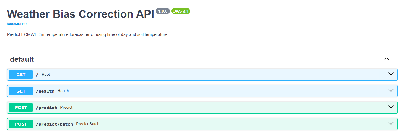
A trained model in a models/ folder is not yet a product. The inference layer exposes a REST API:

Example request:

Example response:

The API loads the serialized model at startup via FastAPI’s lifespan hook, validates inputs with Pydantic, and returns either the predicted error alone or a fully bias-corrected temperature when raw_forecast_temp is supplied.

Auto-generated docs are available at /docs when the server is running locally:

python run_api.py

# → http://127.0.0.1:8000/docs

Step 5: Deploying to production

The project includes a render.yaml config for deployment on Render:

The server binds to 0.0.0.0 when a PORT environment variable is set — standard for cloud platforms — and falls back to local development on 127.0.0.1:8000.

This closes the loop: live data → trained artifact → HTTP inference → cloud deployment.

What I learned as an AI engineer

1. Domain structure beats model complexity

The win here did not come from a massive deep learning architecture. It came from choosing features that reflect physical error mechanisms — diurnal cycle and land-surface coupling.

2. Pipelines outlive models

Caching, alignment, evaluation baselines, and train/serve feature parity will still matter when you swap Random Forest for XGBoost or a neural net. Build the skeleton first.

3. Visual diagnostics build trust

The diurnal plot and interaction heatmap are not garnish. They explain why the model works and give scientists and engineers a shared language for validation.

4. Production ML is correction, not replacement

The most impactful AI systems in weather today often sit downstream of physics, not upstream of it. That is a feature, not a limitation.

Where this could go next

This project opens several natural extensions:

• More features — elevation, vegetation, season, forecast lead time, humidity
• Per-station or clustered models — localized bias regimes
• Probabilistic output — quantile regression or ensemble post-processing for uncertainty
• Automated retraining — scheduled pipeline runs as new ECMWF data arrives
• Monitoring — drift detection on feature distributions and error metrics in production

The current system is intentionally lean. That is the right starting point.

Conclusion

Numerical weather prediction is one of humanity’s great scientific achievements. But “great” is not the same as “finished.” Systematic bias still leaks through — in the dawn hour, at the land surface, in the gap between grid box and station reality.

This project demonstrates a practical path forward: learn the error, subtract the error, serve the correction.

Five million data points. Two interpretable features. One Random Forest. One FastAPI service. About seven percent better.

In AI engineering, especially in domains that matter, that is exactly the kind of win worth shipping.

🔗 Links

• GitHub: https://github.com/ChristechAnalytics/weather_bias_prediction
• Live API docs: https://weather-bias-prediction.onrender.com/docs