Molecular Docking Made Easy: A Step-by-Step Guide to AutoDock4 using AutoDockTools

Introduction

Molecular docking is a key technique in computational drug discovery. It predicts the preferred orientation of a ligand (usually a small molecule drug) when bound to a target protein (receptor), helping scientists understand binding affinity and interaction patterns.

In this article, I walk you through a complete and error-free molecular docking pipeline using AutoDock4 and AutoDockTools (ADT) on Windows. This guide is tailored for practical sessions, academic projects, and personal exploration in structure-based drug design.

By the end of this guide, you’ll be able to:

• Prepare receptor and ligand files properly.
• Set up grid and docking parameter files (GPF/DPF).
• Run AutoGrid and AutoDock using the correct command-line syntax.
• Visualize and interpret docking results confidently.

We’ll not just “do the steps”, but understand why each step is done. This is crucial for avoiding common errors (like missing .Cl.map files), interpreting results meaningfully, and performing high-quality docking simulations.

🧰 Prerequisites

• AutoDock4 and AutoDockTools (ADT) installed on your Windows system
• Receptor and Ligand structures (in .pdb format)
• Basic familiarity with molecular structures (proteins and ligands)

Let’s begin with the first and most critical part — preparing the receptor.

You’re starting off with a protein-ligand complex (PDB ID: 8XR5) and will extract the receptor and ligand using PyMOL

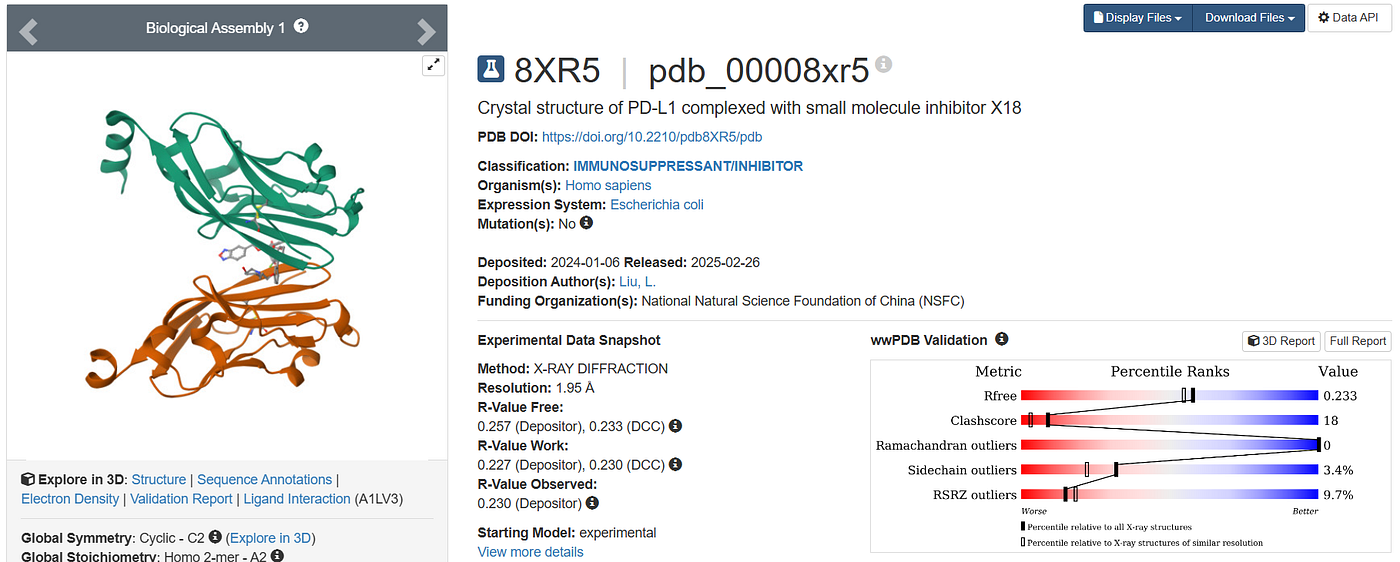
Fig 01. We will be downloading and using this RCSB PDB Receptor Ligand Complex. Here the standard PDB format is not available so we use the .cif complex strucutre. Go to → Download Files → PDBx/mmCIF Format.

🧩 Section 1: Extracting Receptor and Ligand from the Protein-Ligand Complex using PyMOL

Most protein-ligand complexes from the PDB are experimental crystal structures. These contain not just the protein and ligand but also:

• Water molecules (HOH)
• Metal ions
• Buffers or solvents (e.g., SO4, GOL)
• Sometimes, multiple chains and ligands

If you directly use such files for molecular docking in AutoDock without preprocessing:

• You’ll get mapping errors (e.g., .Cl.map missing)
• Incorrect grid box size or placement
• Wrong docking results due to extra atoms interfering

Thus, the first and most important step is to separate:

• Receptor → the protein (without water, cofactors, etc.)
• Ligand → the small molecule inhibitor

🧪 Tools Needed: **PyMOL (open-source or educational license)**

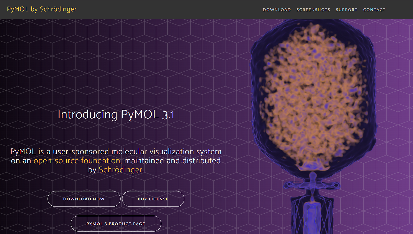
Fig 02. Pymol 3D molecular Visualization Tool 3.1 as of the writing of this article.

Here, once you have installed the Pymol software, depending on the version of your Operating system, open the software, and here you will see this window.

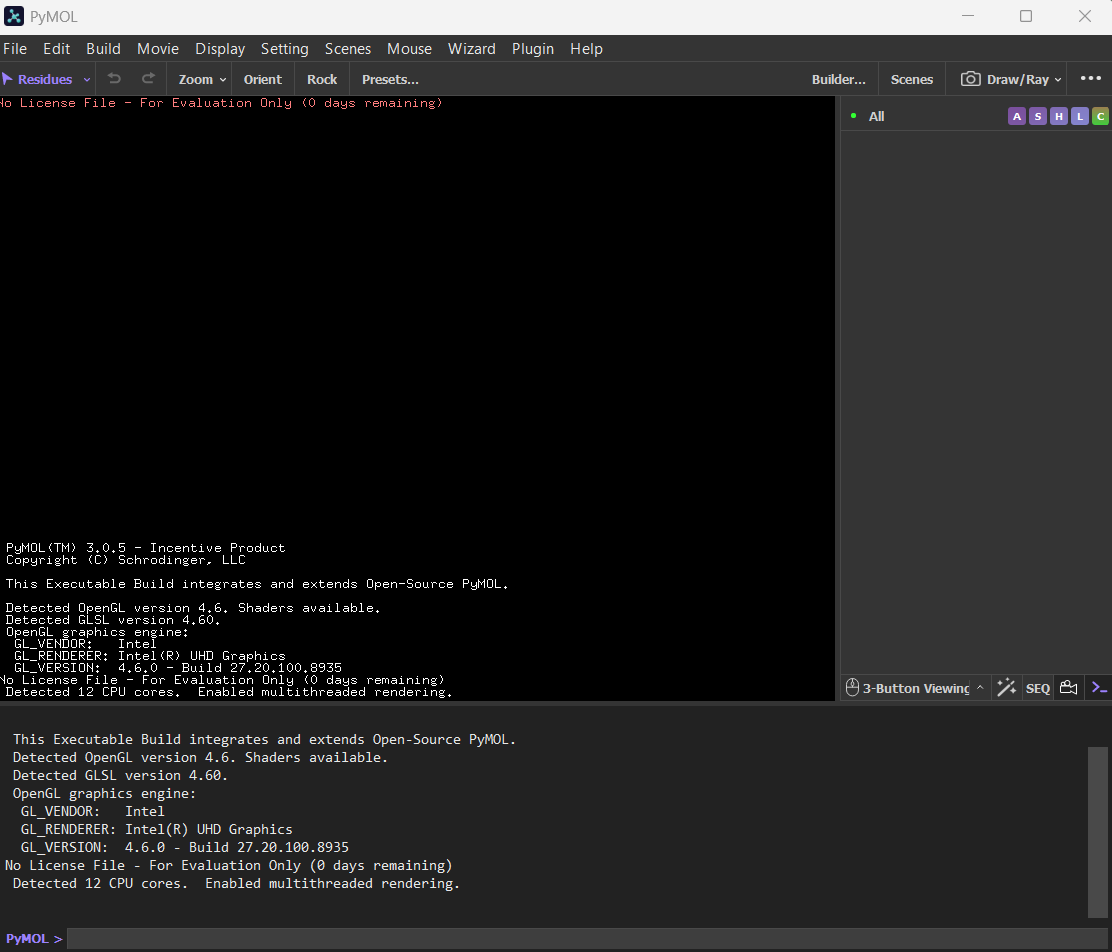
Fig 03. Typical outlay of the pymol workspace intially.

Type Fetch “8XR5” into the pymol terminal to load the protein-ligand complex

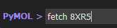
Fig 04. Pymol terminal fetches the strucutre directly from PDB.

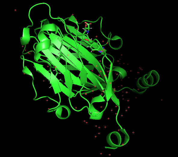
Fig 05. Crystal structure of PD-L1 complexed with small molecule inhibitor X18 viewed in the pymol main view window pane.

Click on “All” from the right-hand pane window view and

go to “Action” → ”Remove Waters”

This will get rid of the water molecules

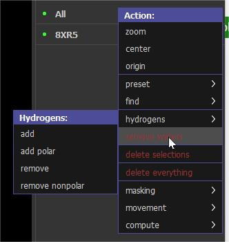
Fig 06. This option would remove all waters

👣 Step-by-Step Guide Using PyMOL GUI

Open the Sequence Viewer Using the SEQ Button To make selection easier, we’ll open the sequence viewer inside PyMOL:

Look at the right panel where your object is loaded (e.g., 8xr5 or similar).

Click the SEQ button next to your object. This opens a linear sequence view of your protein, showing chains and ligands.

This viewer displays all residues, including standard amino acids (like ALA and GLY) and non-standard entries (like ligands and cofactors). It’s a convenient way to select only what you need visually.

Export the Protein (Receptor Only)

Once the SEQ viewer is open, follow these steps:

Click and drag to select the amino acid sequence of your desired protein chain(s). For example, if your structure has chains A and B that form the protein, select both if needed.

With the protein sequence selected, go to:

File → Export Structure → Export Molecule

A dialog box will open. Save the file as:

receptor.pdb

💡 Make sure only the protein chain(s) are selected. Avoid selecting heteroatoms like water (HOH), ions, or ligands.

Export the Ligand

Now, let’s isolate and save the ligand molecule separately:

In the SEQ viewer or the 3D view, locate the ligand — typically labeled with a 3-letter code (like X18, LIG, or INH).

Click on it to highlight and select the ligand.

>> File → Export Structure → Export Molecule

>> ligand.pdb

You can verify it’s correct by loading the saved file back into PyMOL — it should only contain the small molecule with no protein residues.

🎯 Final Output Recap

You should now have:

receptor.pdb — the clean protein structure, ready for docking

ligand.pdb — the isolated small molecule for docking

🧩 Section 2: Preparing the Receptor in AutoDockTools (ADT) the Right Way

Once we’ve extracted the receptor (protein structure) from the complex using PyMOL, the next step is to prepare it for docking in AutoDock. This involves converting the .pdb file to a .pdbqt format using ADT, with proper hydrogens, charges, and AD4-specific atom typing.

🔹 1. Load the Receptor

File → Read Molecule → receptor.pdb

✅ You should see the protein model appear in the viewer. If not, check your .pdb file for formatting errors.

🔹 2. Add Polar Hydrogens

Edit → Hydrogens → Add → Polar Only

Why this step? Docking simulations rely heavily on hydrogen bonding interactions. We add polar hydrogens (those bound to electronegative atoms like N and O) as they participate in such interactions.

🔹 3. Assign Gasteiger Charges

Edit → Charges → Compute Gasteiger

These partial atomic charges are necessary for calculating electrostatic interactions during docking.

🔹 4. Assign AD4 Atom Types (🛑 Commonly Forgotten but Critical)

Edit → Atom Types → Assign AD4 Types

Why this step is vital: AutoDock4 needs each atom labeled with a specific atom type (like A, C, HD, OA, Cl, etc.). If you forget this, you’ll later get an error like:

FATAL ERROR: cannot find receptor.Cl.map

This step ensures that map files will be correctly generated in the grid preparation phase.

🔹 >5. Define Macromolecule for Grid Mapping

Grid → Macromolecule → Choose…

→ Select the currently loaded receptor molecule.

Why this matters: This tells ADT that this molecule is the target (macromolecule) and that grid maps will be generated around it.

You’ll see a confirmation in the terminal like:

Set receptor filename to: receptor.pdbqt

🔹 6. Save the Receptor as PDBQT

File → Save → Write PDBQT

→ Name the file receptor.pdbqt.

This is the final processed receptor file you’ll need for grid and docking steps.

🧩 Section 3: Preparing the Ligand for Docking in AutoDockTools (ADT)

Now that our receptor is ready let’s prepare the ligand, the small molecule that will bind to the target protein. This step ensures that the ligand is chemically correct, flexible (with defined rotatable bonds), and ready for docking using AutoDock4.

We’ll be working with the Ligand.pdb file that we extracted earlier using PyMOL.

🔹 1. Load the Ligand Molecule

File → Read Molecule → Ligand.pdb

You should see a smaller molecule loaded in the viewer, typically colored differently from the receptor.

🔹 2. Add All Hydrogens

Edit → Hydrogens → Add → All Hydrogens

Why this step? Unlike the receptor where we add polar hydrogens only, ligands need all hydrogens — polar and nonpolar — to be chemically complete and to avoid valency errors in torsion tree calculations.

🔹 3. Compute Gasteiger Charges

Edit → Charges → Compute Gasteiger

Gasteiger charges are used to calculate electrostatic interactions in AutoDock’s scoring function. This is essential before generating the .pdbqt.

🔹 4. Detect Torsions (Flexibility)

Ligand → Torsion Tree → Detect Root

Then:

Ligand → Torsion Tree → Define Rotatable Bonds

Why this step matters: The torsion tree defines which parts of the ligand can rotate (i.e., flexible bonds). AutoDock will use this information during the search to explore different ligand conformations.

• The root is the central, usually largest, rigid part of the ligand.
• The rotatable bonds allow the molecule to fit into the receptor’s binding pocket flexibly.

You’ll see yellow arrows on rotatable bonds in the viewer if this is done properly.

🔹 5. Save the Ligand as PDBQT

File → Save → Write PDBQT

→ Save the file as: Ligand.pdbqt

This is now your ready-to-dock ligand, complete with charges and flexibility.

✅ Final Checkpoint

At this point, your working directory should now have:

• Ligand.pdbqt
• receptor.pdbqt

Both are properly prepared and will be used to:

1. Generate the grid parameter file (.gpf)
2. Run autogrid4.exe to create the map files
3. Prepare the docking parameter file (.dpf)
4. Execute docking with autodock4.exe

🧩 Section 4: Setting Up Grid Parameters (.GPF) in AutoDockTools

Before docking can be performed, AutoDock needs to precompute a set of energy interaction maps, which help efficiently evaluate the binding affinity between the ligand and receptor. This is done by configuring a grid box and generating a Grid Parameter File (GPF).

🔹 1. Set Map Types Based on Ligand Atoms

Grid → Set Map Types → Choose Ligand…

Choose Ligand.pdbqt from the dialog.

Why this step? This tells AutoDock which atom types (C, N, O, Cl, Br, etc.) are present in the ligand, so it can create corresponding interaction map files. If you skip this, you may encounter errors like:

FATAL ERROR: can't find or open "receptor.Cl.map"

This ensures maps are created for all atoms the ligand might have.

🔹 2. Define the Grid Box Around Active Site

Grid → Grid Box

You’ll now see a 3D box overlayed on the receptor in the AutoDockTools viewer.

Adjust the Box:

• Use the mouse or number input to center it over the active site or binding pocket.
• Adjust grid size (number of points in x, y, z) to ensure the ligand has enough space to explore conformations.

Why it matters: The grid box defines the search space. If it’s too small, your ligand may not find the best pose. If it’s too big, docking may become inefficient.

🧠 Tip: If unsure where the binding site is, you can center the box on the ligand’s original position (if working from a complex).

🔹 3. Save the Grid Parameter File

Grid → Output → Write GPF

Save it as:

grid.gpf

This .gpf file contains all the map configuration settings: receptor, ligand atom types, box dimensions, and map spacing.

Summary

You’ve now prepared the configuration that will be used to generate energy maps for docking. You should now have:

• grid.gpf — grid parameter file
• All necessary .pdbqt files from earlier steps

Next, we’ll generate the grid maps using the autogrid4.exe tool in the terminal.

Important Note

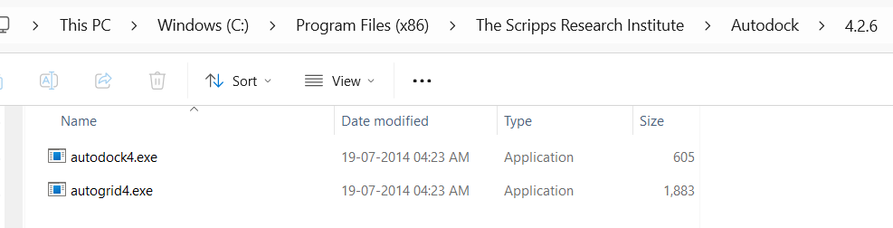
The autodock4 and autogrid4 exe files have to be copied into you working directory where the pdbqt files along with the .dpf and .gpf files for successful execution of the docking simulation.

Do not forget to copy these files into your working directory; otherwise, the commands will not run in the command-line interface.

🧩Section 5: Running AutoGrid (Generate Receptor Maps)

Once the Grid Parameter File (.gpf) is set, you’ll need to run AutoGrid, a key pre-processing step that computes grid maps for the receptor based on the ligand’s atom types. These maps are essential for efficient docking.

🔹 1. Open PowerShell or CMD

Navigate to the folder where your files (grid.gpf, receptor.pdbqt, etc.) are located.

Example:

cd "C:\Users\Downloads\Practical"

🔹 2. Run the AutoGrid Command

Execute the following in PowerShell or CMD:

.\autogrid4.exe -p grid.gpf -l grid.glg

• -p → specifies the input grid parameter file (grid.gpf)
• -l → specifies the output log file (grid.glg) for checking the process

What Should Be Generated

Upon successful execution, you should see a series of map files:

• receptor.C.map, receptor.OA.map, receptor.N.map, receptor.HD.map, etc. (based on atom types in your ligand)
• receptor.Cl.map, receptor.Br.map if Cl or Br atoms are in the ligand
• receptor.maps.fld → field file summarizing all map data
• receptor.maps.xyz → coordinate file used for grid placement

💡 Why are these important? These .map files allow AutoDock to rapidly score ligand poses during docking, by reusing precomputed receptor interaction energies.

❗ Common Pitfall: Missing .map Files

If you skipped setting map types based on the ligand (in the previous step), AutoGrid might throw an error like:

FATAL ERROR: can't find or open receptor.Cl.map

Fix this by revisiting:

Grid → Set Map Types → Choose Ligand…

and re-saving your grid.gpf.

With AutoGrid completed, the receptor is fully preprocessed and ready for the docking simulation.

🧩Section 6: Prepare Docking Parameters (.DPF)

Once your ligand and receptor are ready in .pdbqt format and the receptor maps are generated via AutoGrid, the next step is to generate a Docking Parameter File (.dpf). This file contains all the configuration settings AutoDock4 will use to perform docking.

We will do this step-by-step via the AutoDock Tools (ADT) interface.

🔹 1. Load the Ligand for Docking

From the ADT menu:

*Docking → Ligand → Choose… Select your ligand file: 🧾 Ligand.pdbqt*

🔹 2. Load the Receptor (Macromolecule)

*Docking → Macromolecule → Set Rigid Filename… Select: 🧾 receptor.pdbqt*

Why this? You are specifying the receptor AutoDock should dock against, and treating it as rigid (as typical in most docking setups).

🔹 3. Set Search Parameters

*Docking → Search Parameters → **Choose…***

• The Lamarckian Genetic Algorithm (LGA) is used by default, which is good.
• You can leave all the default values for most cases:
• 10 GA runs
• 150 population size
• 2,500,000 evals (adjustable for accuracy/speed tradeoff)

✅ Why LGA? It’s a robust hybrid algorithm that combines genetic and local search methods for efficient exploration and refinement of binding poses.

🔹 4. Docking Parameters (Optional Check)

*Docking → Docking Parameters*

Here, ensure:

• The ligand and receptor are properly defined.
• The grid maps match the atom types of your ligand.
• You should see a list of .map files like receptor.C.map, receptor.N.map, etc.

⚠️ Be careful here! If you missed assigning AD4 types or forgot setting map types, you’ll get errors during docking like “can’t find receptor.Cl.map”.

🔹 5. Select Docking Algorithm

*Docking → Output → **Lamarckian Genetic Algorithm***

This sets the algorithm to be used in the .dpf file. You can optionally choose Simulated Annealing or Genetic Algorithm alone, but LGA is typically preferred.

🔹 6. Save Docking Parameters File

*Docking → Output → **Write DPF***

Save the file as: 🧾 dock.dpf

This file combines all your docking configurations and will be used by AutoDock in the next step.

📌 Summary of Files So Far:

Ligand.pdbqtPrepared ligand file

receptor.pdbqtPrepared receptor (rigid)

grid.gpfGrid parameters (for AutoGrid)

grid.glgAutoGrid log file

receptor.*.mapGrid maps for each ligand atom type

receptor.maps.fldMap field summary

dock.dpfDocking configuration (for AutoDock)

🧩Section 7: Run AutoDock 4 for Docking

Now that you have your docking parameter file (dock.dpf) ready, it's time to execute the docking run using AutoDock4 from the command line.

This will simulate the ligand binding to the receptor using the parameters you set up earlier and output a docking log file (dock.dlg) that contains all the results.

🔹 1. Open PowerShell or CMD

Navigate to the folder where all your prepared files are located — this should include:

• dock.dpf
• Ligand.pdbqt
• receptor.pdbqt
• All required receptor.*.map files
• receptor.maps.fld

🔹 2. Run AutoDock Command

In the terminal, run the following:

.\autodock4.exe -p dock.dpf -l dock.dlg

Where:

• -p dock.dpf → specifies the docking parameter file
• -l dock.dlg → names the output docking log file

Make sure autodock4.exe is in the same directory or added to your system PATH.

🔍 What Happens Next?

AutoDock will begin the docking run, showing output like:

AutoDock 4.2.6
... Running Lamarckian Genetic Algorithm ...
... Evaluating binding poses ...
... Writing results to dock.dlg ...

This process might take anywhere from a few seconds to several minutes, depending on the following:

• Ligand size
• Receptor complexity
• Number of GA runs and evaluations

✅ Output Files

After successful execution, you’ll have:

FileDescriptiondock.dlgDocking log file — primary result fileLigand.pdbqtThe ligand you dockedreceptor.pdbqtThe receptor useddock.dpfDocking parameters usedreceptor.*.mapPrecomputed maps from AutoGrid

🔍 What’s Inside dock.dlg?

This file contains:

• 🧠 Predicted binding energies (ΔG)
• 📍 Final docked conformations (poses)
• 🔁 Number of GA runs & clusters
• 🔒 Docking success messages and log details

You’ll later open this file in AutoDock Tools to visualize the binding poses and energies.

Pro Tip: If you see errors like:

FATAL ERROR: can't find receptor.Cl.map

This usually means:

• You didn’t assign AD4 atom types to the receptor
• Or you didn’t select the ligand when setting map types in the Grid menu

Always go back and double-check the steps if this occurs.

🧩Section 8: Analyze Docking Results in AutoDock Tools (ADT)

After you’ve successfully run autodock4.exe, the results are stored in the dock.dlg file. This file contains valuable information like binding energies, ligand poses, and docking clusters.

Let’s explore how to open and understand this file using AutoDock Tools.

🔹 1. Open dock.dlg in ADT

In AutoDock Tools:

• Go to Analyze → Dockings → Open…
• Select your docking log file → dock.dlg

💡 This tells ADT to parse all docking runs, poses, and energies for further analysis.

🔹 2. Examine Docking Conformations

Once dock.dlg is loaded:

• Navigate to Analyze → Conformations
• Use the following options:
• Show Info: View binding energies and pose info
• Play: Cycle through different poses
• Cluster: View pose clustering by RMSD

Fig 07. This view pane shows the different poses generated by the autodock4.

This helps you:

• See the top-ranked docking poses
• Identify most stable conformations
• Understand binding affinity scores (lower = better)

[embed]

🧾 Conclusion: Your End-to-End AutoDock 4 Workflow

In this practical guide, we walked through the complete molecular docking pipeline — from preparing PDB files using PyMOL, to generating .pdbqt files with AutoDock Tools, configuring grid and docking parameters, running simulations via AutoGrid and AutoDock, and finally analyzing results to interpret binding affinities and pose clusters.

Why This Matters:

• Accurate receptor and ligand preparation is crucial to avoid common errors like missing .Cl.map files.
• Assigning AD4 atom types ensures the docking engine recognizes all atoms.
• Properly setting the grid box ensures the docking explores the right region — the active site.
• Understanding docking results visually and numerically helps assess the biological relevance of the interaction.

Key Takeaways:

• Always verify each step (hydrogens, charges, torsions, atom types).
• Use PyMOL’s SEQ button and export carefully to get clean receptor/ligand files.
• Keep AutoDock tools and input files in one directory for easier execution.
• Double-check grid and docking parameter files to align with the ligand’s atom types.

📚 Ready for Practicals and Research

With this workflow, you can confidently demonstrate docking simulations in practical exams or use them in research.

✉️ Have questions or want to automate parts of this workflow? Reach out or drop a comment on the article! 🧪 *Happy Docking!*

🎉 You’re now ready to perform and present molecular docking using AutoDock 4 confidently!

[embed]Download AutoDock4 AutoDock 4.2.6 Download Page AutoDock is distributed freely under the GNU GPL for all to use.autodock.scripps.edu