Deep Dream: Visualizing the features learnt by Convolutional Networks in PyTorch

Convolutional neural networks (CNNs) are one of the most effective machine learning tools when it comes to computer-vision related tasks. Their effectiveness can be gauged from the fact that most of the computer vision contests such as ILSVRC, PASCAL VOC and COCO have come to be dominated by entries using innovative CNN based architectures to achieve their goals.

It is therefore interesting to ask “what are the features learnt by the various filters in a given CNN?”. Not only is this question interesting from the plain old ‘curiosity’ point of view, but more importantly knowing the answer to this question can give us extremely useful insights into improving the performance of our CNNs. For e.g. the winning entry (Clarifai) from the ILSVRC-2013 challenge was designed by improving the previous year’s winning entry (AlexNet). These improvements were chosen by applying feature-visualization techniques (Deconvnets) on AlexNet. See this paper (by the winners of ILSVRC-2013) for more details or this blog for a nice review.

In this post, we will learn how to visualize the features learnt by CNNs using a technique called ‘activation-maximization’, which starts with an image consisting of randomly initialized pixels whose values are slowly tweaked to maximize the output of the layer we wish to visualize. This was first introduced in this paper and was first applied to CNNs in this paper. A naive application of activation maximization on CNNs, however, tends to produce extremely high-frequency images which looking nothing like the real-world natural images that one comes across on a day to day basis. For e.g see here for a great description of this problem and a discussion of common approaches to solve them. In this post, we will limit ourselves to using three simple regularization techniques to make the images more meaningful:

1. Starting with a small 28 x 28 image and slowly upscaling it to the desired size, for e.g. as done here.
2. Penalizing large pixel-values
3. Penalizing large pixel-gradients in the image i.e. penalizing any sharp changes in the values of neighbouring pixels.

So let’s get started. The complete code containing various things I tried can be found on my Github. This post is based on trial #6 in the notebook. Here I will go over the code in some detail. As an aside, let me mention that recently I also came across a wonderful Keras-implementation of the same technique by Keras creator Francois Chollet. I would highly recommend everyone to take a look at his post.

Let us begin by loading a pretrained model:

import torch
from torchvision import models
model = models.googlenet(pretrained = True)

While most of the blogs on activation maximization that I have seen tend to work with VGG16 as their pretrained model, for no particular reason other than that of trying something different, I will use GoogLeNet. Almost all the code in this blog can be straightforwardly applied to any other pretrained CNN.

Since we are interested in visualizing what the model has learnt rather than re-train the model, we should, therefore, freeze the model parameters so that they do not change during backpropagation.

for param in model.parameters():
    param.requires_grad_(False)

Note that the various layers in the model can be easily accessed via unique names that have been given to them. Let us, therefore, list the names of the different layers in the model:

list(map(lambda x: x[0], model.named_children()))

On GoogLeNet this produces the following output

['conv1',
 'maxpool1',
 'conv2',
 'conv3',
 'maxpool2',
 'inception3a',
 'inception3b',
 'maxpool3',
 'inception4a',
 'inception4b',
 'inception4c',
 'inception4d',
 'inception4e',
 'maxpool4',
 'inception5a',
 'inception5b',
 'avgpool',
 'dropout',
 'fc']

For demonstration purposes here, I will (randomly) choose the layer named ‘inception4a’. We now have to register a forward hook for this layer. Hooks provide easy access to the output and grad_ouput of the desired layer. As the name suggests, a forward hook is executed during the forward pass and allows us to view/modify the output of a layer. Similarly, a backward hook is executed during the backward pass and allows us to view/modify the grad_ouput of a layer. Check out this blog and this kaggle kernel for more on hooks. The implementation here is based on this discussion on pytorch discussion board. To register a forward hook, we first define the following factory function that returns a function object that we will use as our hook:

activation = {} # dictionary to store the activation of a layer

def create_hook(name):
 def hook(m, i, o):
   # copy the output of the given layer
   activation[name] = o

 return hook

We now register the hook:

# register a forward hook for layer inception4a
model.inception4a.register_forward_hook(create_hook(‘4a’))

Note that pretrained models on PyTorch require that input images “ have to be loaded in to a range of [0, 1] and then normalized using mean = [0.485, 0.456, 0.406] and std = [0.229, 0.224, 0.225]”. We will, therefore, define the following transformations on our images:

# normalize the input image to have appropriate mean and standard deviation as specified by pytorch

from torchvision import transforms

normalize = transforms.Normalize(mean=[0.485, 0.456, 0.406],
                                 std=[0.229, 0.224, 0.225])

# undo the above normalization if and when the need arises 

denormalize = transforms.Normalize(mean = [-0.485/0.229, -0.456/0.224, -0.406/0.225], std = [1/0.229, 1/0.224, 1/0.225] )

Let us now define a function to generate an image consisting of randomly initialized pixels. In order to allow for the image to be tweaked during backpropagation, we will have to set the “requiresgrad” flag of the image to be True.

import numpy as np

Height = 28
Width = 28

# generate a numpy array with random values
img = np.single(np.random.uniform(0,1, (3, Height, Width)))

# convert to a torch tensor, normalize, set the requires_grad_ flag
im_tensor = normalize(torch.from_numpy(img)).requires_grad_(True)

Let us also define a function to denormalize the image and move the color channels to the last dimensions in order to display it using matplotlib’s imshow. This will also be handy when resizing images using open-cv’s resize method.

# function to massage img_tensor for using as input to plt.imshow()
def image_converter(im):

    # move the image to cpu
    im_copy = im.cpu()

    # for plt.imshow() the channel-dimension is the last
    # therefore use transpose to permute axes
    im_copy = denormalize(im_copy.clone().detach()).numpy()
    im_copy = im_copy.transpose(1,2,0)

    # clip negative values as plt.imshow() only accepts 
    # floating values in range [0,1] and integers in range [0,255]
    im_copy = im_copy.clip(0, 1) 

    return im_copy

As we had mentioned before, we wish to penalize any sharp changes in pixel values across the image i.e. we will penalize the x- and y-derivatives of the pixel values in the image. This can be done by creating a Convolution layer with either Sobel filters or Scharr filters. We can define a convolutional layer which can accept either of these filters as follows:

import torch.nn as nn

# class to compute image gradients in pytorch
class RGBgradients(nn.Module):
    def __init__(self, weight): # weight is a numpy array
        super().__init__()
        k_height, k_width = weight.shape[1:]
        # assuming that the height and width of the kernel are always odd numbers
        padding_x = int((k_height-1)/2)
        padding_y = int((k_width-1)/2)

        # convolutional layer with 3 in_channels and 6 out_channels 
        # the 3 in_channels are the color channels of the image
        # for each in_channel we have 2 out_channels corresponding to the x and the y gradients
        self.conv = nn.Conv2d(3, 6, (k_height, k_width), bias = False, 
                              padding = (padding_x, padding_y) )
        # initialize the weights of the convolutional layer to be the one provided
        # the weights correspond to the x/y filter for the channel in question and zeros for other channels
        weight1x = np.array([weight[0], 
                             np.zeros((k_height, k_width)), 
                             np.zeros((k_height, k_width))]) # x-derivative for 1st in_channel

        weight1y = np.array([weight[1], 
                             np.zeros((k_height, k_width)), 
                             np.zeros((k_height, k_width))]) # y-derivative for 1st in_channel

        weight2x = np.array([np.zeros((k_height, k_width)),
                             weight[0],
                             np.zeros((k_height, k_width))]) # x-derivative for 2nd in_channel

        weight2y = np.array([np.zeros((k_height, k_width)), 
                             weight[1],
                             np.zeros((k_height, k_width))]) # y-derivative for 2nd in_channel


        weight3x = np.array([np.zeros((k_height, k_width)),
                             np.zeros((k_height, k_width)),
                             weight[0]]) # x-derivative for 3rd in_channel

        weight3y = np.array([np.zeros((k_height, k_width)),
                             np.zeros((k_height, k_width)), 
                             weight[1]]) # y-derivative for 3rd in_channel

        weight_final = torch.from_numpy(np.array([          weight1x, weight1y, 
weight2x, weight2y,
weight3x, weight3y])).type(torch.FloatTensor)

        if self.conv.weight.shape == weight_final.shape:
            self.conv.weight = nn.Parameter(weight_final)
            self.conv.weight.requires_grad_(False)
        else:
            print('Error: The shape of the given weights is not correct')

    # Note that a second way to define the conv. layer here would be to pass group = 3 when calling torch.nn.Conv2d

    def forward(self, x):
        return self.conv(x)

Turns out, for 3 x 3 kernels, Scharr filters are better then Sobel filters, therefore we will use Scharr filters:

# Scharr Filters

filter_x = np.array([[-3, 0, 3], 
                     [-10, 0, 10],
                     [-3, 0, 3]])

filter_y = filter_x.T
grad_filters = np.array([filter_x, filter_y])

Let us now create an instance of the above-defined convolutional layer by passing it the Scharr filters.

gradLayer = RGBgradients(grad_filters)

Let us also define a function that uses the above-defined gradLayer to compute the x- and y-derivatives of an input image and return their root-mean-squared value.

# function to compute gradient loss of an image 

def grad_loss(img, beta = 1, device = 'cpu'):

    # move the gradLayer to cuda
    gradLayer.to(device)

    gradSq = gradLayer(img.unsqueeze(0))**2

    grad_loss = torch.pow(gradSq.mean(), beta/2)

    return grad_loss

Finally, let us move everything to the GPU. You can skip the following step if you don’t have a GPU or if you wish to carry out your computations on your cpu.

device = torch.device('cuda' if torch.cuda.is_available() else 'cpu')
print('Calculations being executed on {}'.format(device))

model.to(device)
img_tensor = im_tensor.to(device)

As we, had mentioned earlier, we will also slowly upscale the image. We will do this using opencv’s resize() method (you can also use torchvision.transforms.resize() , if you wish). We, therefore, need to import cv2. We will also need matplotlib.pyplot and torch.optim.

import cv2
from torch import optim
import sys
import matplotlib.pyplot as plt

We are now ready to tweak our random image towards an image that maximizes the output of the chosen node of our convolutional layer. For purposes of this post, let me choose the node having an index value 225.

I will optimize the image for 20 iterations before rescaling by a factor of 1.05. I will repeat this cycle 45 times to give me a final image of size 249 x 249.

unit_idx = 225 # the neuron to visualize
act_wt = 0.5 # factor by which to weigh the activation relative to the regulizer terms

upscaling_steps = 45 # no. of times to upscale
upscaling_factor = 1.05
optim_steps = 20# no. of times to optimize an input image before upscaling

We will now run two nested loops to optimize our image and then upscale it as follows:

model.eval()
for mag_epoch in range(upscaling_steps+1):
    optimizer = optim.Adam([img_tensor], lr = 0.4)

    for opt_epoch in range(optim_steps):
        optimizer.zero_grad()
        model(img_tensor.unsqueeze(0))
        layer_out = activation['4a']
        rms = torch.pow((layer_out[0, unit_idx]**2).mean(), 0.5)
        # terminate if rms is nan
        if torch.isnan(rms):
            print('Error: rms was Nan; Terminating ...')
            sys.exit()

        # pixel intensity
        pxl_inty = torch.pow((img_tensor**2).mean(), 0.5)
        # terminate if pxl_inty is nan
        if torch.isnan(pxl_inty):
            print('Error: Pixel Intensity was Nan; Terminating ...')
            sys.exit()

        # image gradients
        im_grd = grad_loss(img_tensor, beta = 1, device = device)
        # terminate is im_grd is nan
        if torch.isnan(im_grd):
            print('Error: image gradients were Nan; Terminating ...')
            sys.exit()

        loss = -act_wt*rms + pxl_inty + im_grd        
        # print activation at the beginning of each mag_epoch
        if opt_epoch == 0:
            print('begin mag_epoch {}, activation: {}'.format(mag_epoch, rms))
        loss.backward()
        optimizer.step()

    # view the result of optimising the image
    print('end mag_epoch: {}, activation: {}'.format(mag_epoch, rms))
    img = image_converter(img_tensor)    
    plt.imshow(img)
    plt.title('image at the end of mag_epoch: {}'.format(mag_epoch))
    plt.show()

    img = cv2.resize(img, dsize = (0,0), 
                     fx = upscaling_factor, fy = upscaling_factor).transpose(2,0,1) # scale up and move the batch axis to be the first
    img_tensor = normalize(torch.from_numpy(img)).to(device).requires_grad_(True)

In the above code snippet, we have defined three kinds of contributions to the loss function:

1. rms: This is the root-mean-squared value of elements in the output tensor produced by our chosen convolutional unit. We wish to maximize this.
2. pxl_inty: This is the root-mean-squared value of the pixel values in our image. For regularization purposes, we wish to penalize large pixel values and hence keep pxl_inty low.
3. im_grd: This is the root-mean-squared value of the x- and y-derivates of pixel values. By keeping this low, we ensure that there are no sharp changes in the pixel values.

The loss function is therefore given by

loss = -act_wt*rms + pxl_inty + im_grd

Where ‘act_wt’ is the weight we assign to ‘rms’ relative to pxl_inty and im_grd. Changing act_wt, therefore, changes the importance of the unit’s activation in comparison to the pixel intensities and gradients in the image. We also check if at any point of iteration any of these become nan’s, in which case we terminate the code.

Note that in the outer loop i.e. upscaling-loop, each time we resize the image, we generate a new img_tensor, therefore, we have to reconstruct our optimizer at the beginning of each magnification epoch.

Voilà! We are done. Executing the loop above produces the following images:

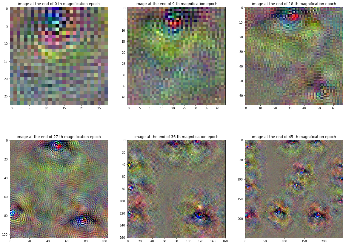
top-left to bottom-right: Images at the end of 0th, 9th, 18th, 27th, 36th and 45th magnification epochs

If I am not biased, then the final image so produced seems to contain a lot of eye-like features. Therefore, we can infer that the convolutional unit in question here must be looking for ‘eyes’ in the input image. It will be fun to see what do other convolutional nodes end up learning. Following are the visualizations for the top 10 most activated units in each layer:

It looks like most of the units in a CNN end up learning different kinds of textures. Occasionally, there are units that seem to learn facial features such as eyes etc. I am not sure why, but to me, it looks like the units in layers inception4a-inception4e and inception5a have the most discernable features. It has been argued in multiple places that the higher layers in CNN end up learning the content of images used to train then as opposed to the lower layers which end up learning their texture. From this point of view, I would expect the last layers, i.e. inception5b to produce images containing highly pronounced humanly interpretable components. However, this does not seem to be the case with the corresponding images mostly containing very high-frequency patterns. Perhaps, I should try a gradient layer with bigger than 3 x 3 filters. Mahendran and Vedaldi had also advocated the use of jitter to regularize the occurrence of these high-frequency patterns. This is something, I have not included here but will be interesting to try.

Hope you will have as much fun with this as I did. 😃