MATHEMATICS EXPLAINED

The Three Moves That Tamed Mathematical Knots

How Kurt Reidemeister Gave Tangled Loops a Grammar

Imagine someone gives you two drawings of a tangled loop.

In the first drawing, the loop twists over itself again and again. In the second, it looks completely different. The crossings are in other places. The shape has been stretched. Some parts are pulled wide, others squeezed close together.

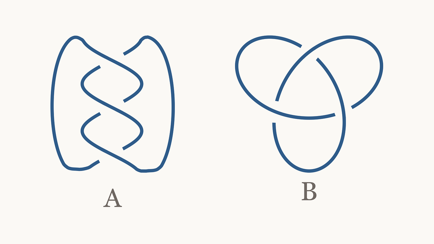
Two different diagrams of the same trefoil knot. Knot theory asks what can change in a drawing while the underlying closed loop remains unchanged.

Then comes the question:

Are these two different knots, or are they the same knot drawn in two different ways?

At first, this sounds like a puzzle about eyesight. Look carefully enough, perhaps, and the answer will reveal itself. But knot theory quickly teaches a harder lesson. Drawings can lie. A knot can be twisted, stretched, rotated, flattened, and redrawn until its appearance changes completely, while the knot itself remains the same.

The problem is not how the knot looks.

The problem is what can be changed without cutting the loop.

Nearly a century ago, the German mathematician Kurt Reidemeister showed that this visual chaos obeys a surprisingly small grammar. Every legitimate change in a knot diagram can be built from three local actions: adding a twist, introducing or removing a pair of crossings, or sliding a strand across a crossing.

With those three moves, knot theory became something much more rigorous than a collection of tangled pictures.

The Problem With A Closed Loop

The knots of mathematics are not quite the knots of daily life.

A shoelace knot has loose ends. A sailor’s knot has loose ends. A cable tangled behind a desk usually has loose ends too, which means the knot can often be undone by pulling one end through the mess.

Mathematical knots remove that possibility.

Take a piece of string. Tie a knot in it. Then join the two ends together. Now there are no loose ends. The knot has become a closed loop in three-dimensional space.

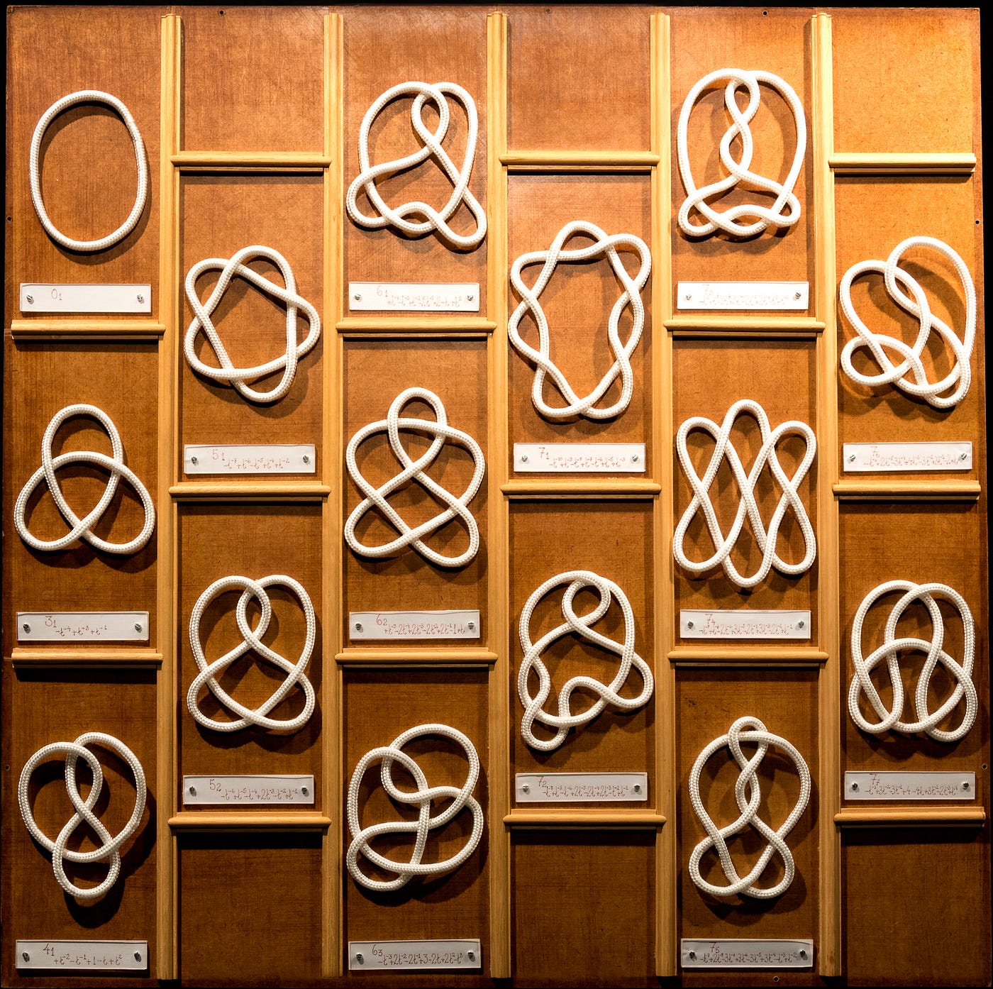
Examples of different knots including the unknot (top left) and the trefoil knot (below it). Exhibit made by Estes Objethos Atelier; photo by Rodrigo Tetsuo Argenton / Matemateca (IME USP), via Wikimedia Commons, licensed under CC BY-SA 4.0.

This small change is essential. Once the ends are joined, the only allowed operations are continuous deformations. You may stretch the loop. You may bend it. You may move it around in space. But you may not cut it, force the string to pass through itself, or open the loop.

The simplest mathematical knot is not really knotted at all. It is just a circle, known as the unknot. It may be stretched into an oval, twisted into a complicated-looking loop, or drawn in a messy way, but if it can be deformed back into a simple circle without cutting, it is still the unknot.

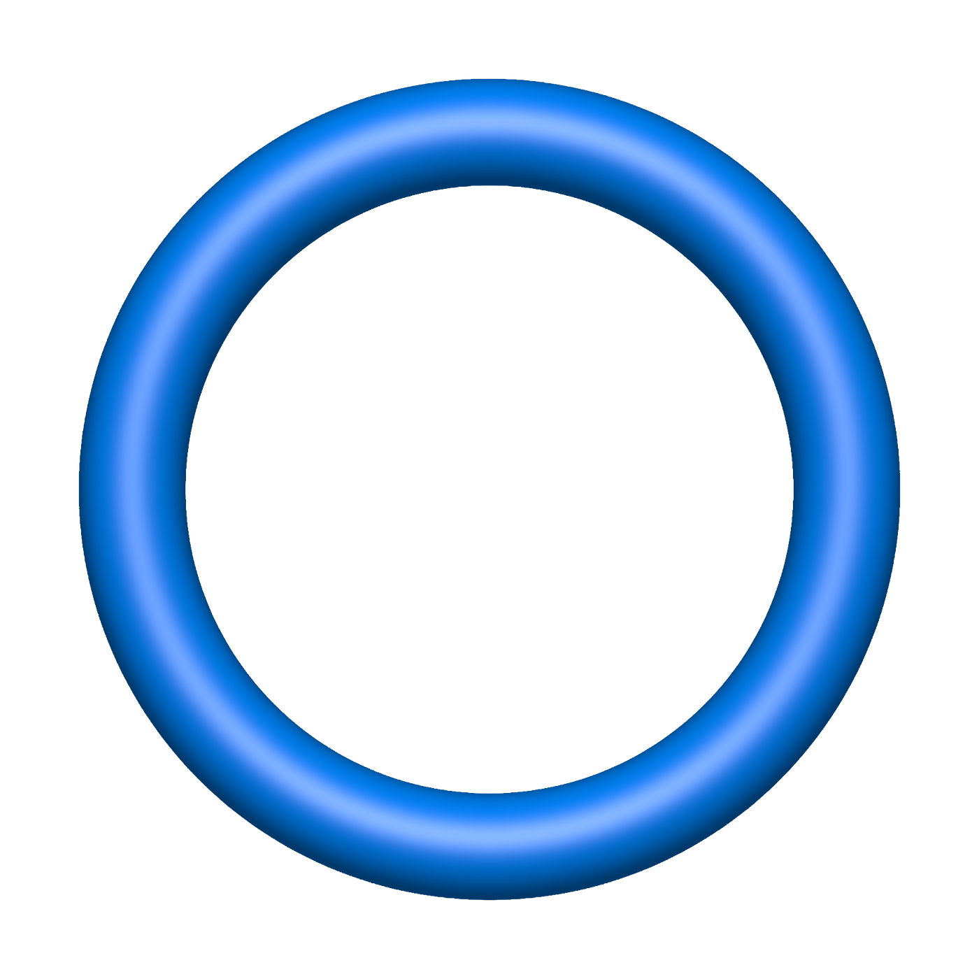
The unknot, the simplest mathematical knot: a closed loop that can be deformed into a circle without cutting. Image by Jim.belk, via Wikimedia Commons, public domain.

The simplest genuinely knotted example is the trefoil knot. It has three crossings in its most economical drawing. It is familiar, compact, and symmetric enough to look almost harmless.

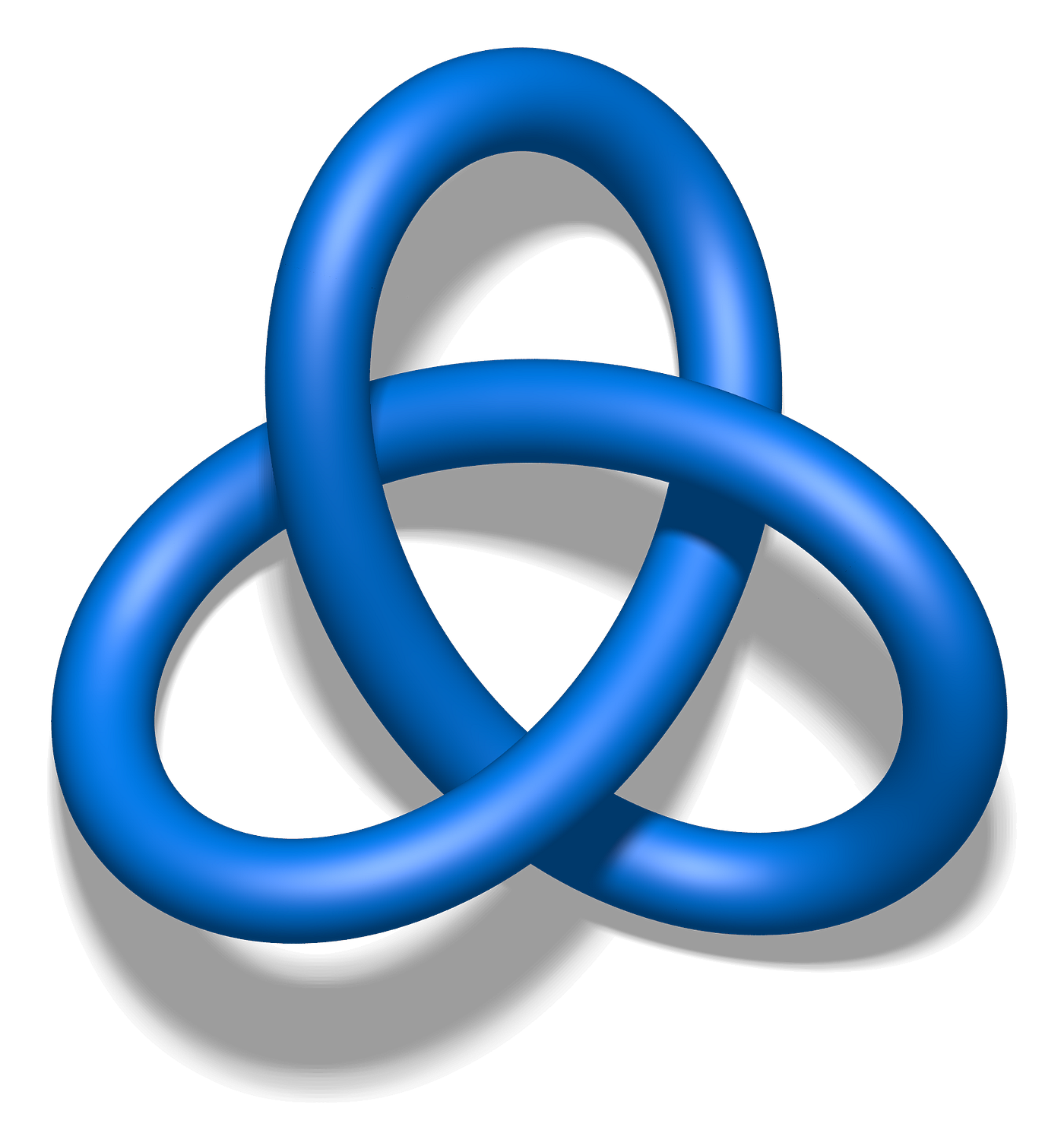
The trefoil knot, the simplest nontrivial mathematical knot. Image by Jim.belk, via Wikimedia Commons, public domain.

But the trefoil cannot be turned into a simple circle without cutting.

That single fact already reveals the central question of knot theory:

How can we tell when two knots are really the same?

A Mathematician Looking For Exact Thought

The mathematician who gave one of the clearest answers to that question was Kurt Werner Friedrich Reidemeister, born in Brunswick, Germany, in 1893.

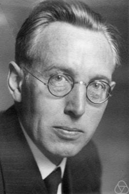
Kurt Reidemeister (1893–1971), about 1930. Photo by L. Reidemeister, Oberwolfach Photo Collection, via Wikimedia Commons, licensed under CC BY-SA 2.0 Germany.

He did not begin as a knot theorist. His intellectual world was unusually broad. In 1920, he passed the Staatsexamen in mathematics, philosophy, physics, chemistry, and geology. He also had strong interests in art history and philosophy.

There was another unusual presence in his early life. Richard Dedekind (1831–1916), one of the great mathematicians of the nineteenth century, was a family friend. Reidemeister called him “uncle”, and Dedekind gave him advice during his school and early university years.

His first research work was far from topology. Reidemeister completed his doctorate in algebraic number theory under Erich Hecke at the University of Hamburg. Then, almost immediately, his mathematical direction changed.

He became interested in geometry, especially through Wilhelm Blaschke. Within a few months of finishing his doctorate, he was already lecturing on differential geometry. The shift was so complete that his doctoral topic became almost an exception in his later work rather than the beginning of a lifelong specialization.

This movement from number theory to geometry to topology matters for the story. Reidemeister was not simply solving a puzzle about string. He was part of a broader transformation in mathematics, where shapes, transformations, groups, and logical foundations were being connected in new ways.

In Vienna, Reidemeister encountered the work of Wilhelm Wirtinger on knots. Wirtinger had shown how algebraic information could be extracted from a knot projection. A drawing of a knot was not merely a drawing. It could encode a group.

Vienna also placed Reidemeister close to Hans Hahn and the intellectual world of the Vienna Circle, where logic, mathematics, language, and scientific knowledge were being examined with unusual intensity. There he did not merely stand near the conversation. He led a group of Vienna mathematicians through a year-long study of Wittgenstein’s “Tractatus”.

This detail matters. Reidemeister’s concern with exactness was not only technical. It belonged to a wider philosophical atmosphere in which mathematicians were asking what it means to reason clearly, to define precisely, and to separate structure from appearance.

His 1926 paper “Knoten und Gruppen” (“Knots and Groups”) already announced the bridge. Knots could be studied through algebraic structure. A few years later, his 1932 book “Knotentheorie” gave one of the early systematic treatments of the subject.

When History Intervened

In 1933, Reidemeister was professor at Königsberg. Shortly before Hitler came to power, National Socialist students caused a disturbance against the university rector. Reidemeister used a mathematics lecture to explain why their behavior was unsupportable and incompatible with rational thought.

Soon after, he was forced out of his chair.

The most striking detail is almost cinematic: he learned of his dismissal from the local newspaper.

Imagine the scene. A professor opens the paper and finds that his academic life has been decided publicly, bureaucratically, and brutally. The dismissal left wounds that, according to later accounts, never fully healed.

Reidemeister’s life reminds us that mathematics is not produced by disembodied minds floating above history. The three moves that bear his name belong to topology, but the man behind them lived through the intellectual brightness of Vienna, the instability of interwar Germany, and the violence of a regime that punished independent judgment.

His most famous mathematical idea asks how apparent disorder can be made exact. To see what he clarified, we have to return from the man to the drawing.

Why Drawings Cannot Be Trusted

Mathematicians usually study knots through diagrams.

A knot lives in three dimensions, but a diagram places it on a flat page. At each crossing, the drawing records which strand passes over and which strand passes under. This over-under information is not decoration. It is part of the knot.

Without it, the drawing would be ambiguous.

But even with this information, a diagram is not the knot itself. It is a projection, a shadow with crossing data attached. The same closed loop may cast many such shadows, depending on how it is positioned before being drawn.

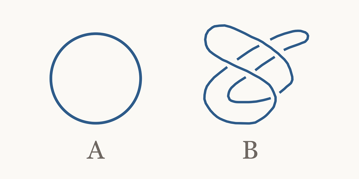
Two projections of the unknot. Diagram A shows the unknot as a simple circle, while diagram B shows the same kind of closed loop drawn with apparent crossings and extra complexity.

So the question becomes sharper. Which changes in the diagram are only changes of viewpoint or deformation, and which changes alter the knot?

Before Reidemeister, this was difficult to formalize. A knot could move in infinitely many ways. It could be pushed, pulled, twisted, and rearranged continuously. How could all those possible motions be captured on a flat page?

Reidemeister’s answer was astonishingly economical.

You do not need infinitely many moves. You need only three.

The Three Moves

A Reidemeister move is a small local change in a knot diagram.

That word “local” is important. The whole knot does not need to be redrawn. Most of the diagram stays untouched. Only a small region changes.

The first move adds or removes a twist.

A strand may curl into a small loop, creating one crossing. Or the loop may be untwisted, removing that crossing. The knot itself has not been cut or changed. Only the diagram has acquired or lost a little curl.

This is Reidemeister Move I.

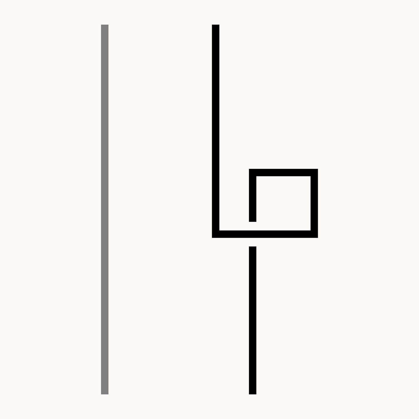
Reidemeister Move I, which adds or removes a small kink in a knot diagram without changing the knot. Image by Parcly Taxel, via Wikimedia Commons, licensed under the Free Art License.

The second move adds or removes two crossings at once.

Imagine one strand passing over another and then back again, creating a pair of crossings. These two crossings can cancel each other when the strands are pulled apart. Conversely, two strands can be pushed together to create such a pair.

This is Reidemeister Move II.

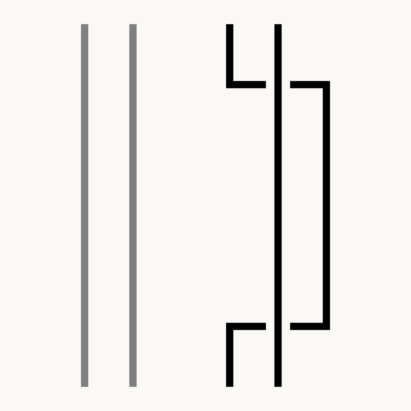
Reidemeister Move II, which adds or removes a pair of crossings without changing the knot. Image by Parcly Taxel, via Wikimedia Commons, licensed under the Free Art License.

The third move slides a strand across a crossing.

In the diagram, one strand moves from one side of a crossing to the other. The number of crossings does not change, but their local arrangement does. It is like moving one piece of string across a small tangle made by two other pieces.

This is Reidemeister Move III.

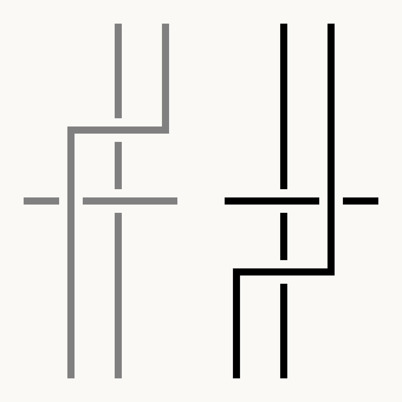
Reidemeister Move III, which slides one strand across a crossing of two other strands without changing the knot. Image by Parcly Taxel, via Wikimedia Commons, licensed under the Free Art License.

Why are there exactly three moves? Because as a knot moves in three-dimensional space, its flat shadow changes smoothly most of the time. The over-under pattern changes only at special instants. A small loop may appear or disappear. Two strands may touch and create, or remove, a pair of crossings. Or one strand may slide across the point where two other strands cross. These are precisely the three local events captured by the Reidemeister moves.

On their own, the moves look almost too simple. They seem like small tricks with diagrams. But together they do something extraordinary.

They describe every possible change of a knot diagram that comes from moving the knot in space. Seen together, the three moves form the small grammar behind the whole theory.

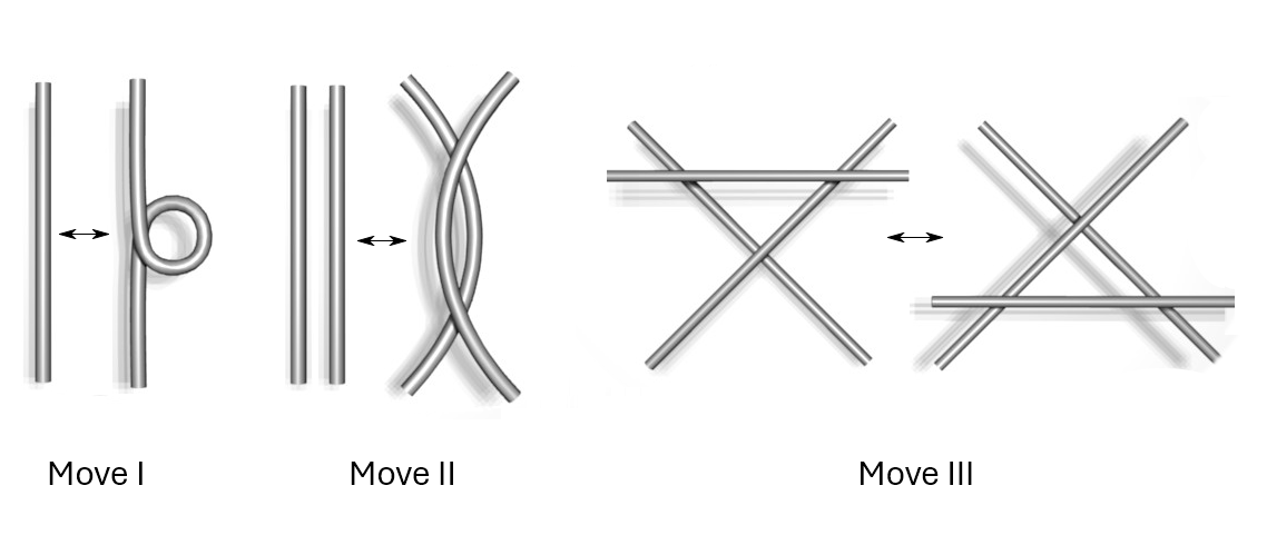
The three Reidemeister moves: adding or removing a twist, adding or removing two crossings, and sliding a strand across a crossing. Composite image based on files by YAMASHITA Makoto, via Wikimedia Commons (I, II, III), licensed under CC BY-SA 3.0, CC BY-SA 2.5/2.0/1.0, and GFDL.

The Theorem Hidden Inside The Moves

The Reidemeister theorem says, roughly, this:

If two diagrams represent the same knot, then one diagram can be transformed into the other by a finite sequence of Reidemeister moves, together with ordinary stretching of the drawing on the plane.

Mathematicians call this ordinary stretching planar isotopy. It means deforming the drawing on the page without creating a new crossing, deleting an old one, or changing which strand passes over another.

The reverse is also true. If one diagram can be transformed into another using Reidemeister moves, then the two diagrams represent the same knot.

Historically, this result was not Reidemeister’s alone. James W. Alexander and Garland B. Briggs independently proved the same diagrammatic principle around the same time. The moves became attached to Reidemeister’s name through his influential treatment of knot theory.

This is the key point.

The moves do not say that every knot can be untangled into a circle. That would be false. The trefoil is not the unknot.

Instead, the theorem says that if two diagrams are merely different drawings of the same knot, then the difference between the drawings can always be explained using these three local moves.

That is a very different claim, and a much deeper one.

It turns a topological problem into a combinatorial one. Instead of thinking about all possible continuous motions of a loop in three-dimensional space, we can think about sequences of moves applied to diagrams.

The knot is still a geometric object. But its transformations now have a language.

A diagram may look complicated. Another diagram may look unrelated. Yet if they represent the same knot, there exists a chain of small diagrammatic steps connecting them.

This is why the Reidemeister moves became foundational. They gave mathematicians a test that any serious knot invariant must pass.

How To Prove A Knot Is Really Different

Suppose someone draws a trefoil knot and asks whether it is really different from the unknot.

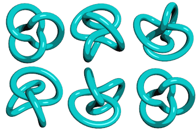
Animated trefoil knot, one of the simplest nontrivial knots. Animation by Philip Rideout, via Wikimedia Commons, licensed under CC BY-SA 3.0.

You try to simplify the diagram. You apply Reidemeister moves. You remove a twist here, slide a strand there, eliminate crossings where you can.

But failure to untangle the diagram is not proof. Maybe you simply have not found the right sequence of moves.

In some cases, even an unknot diagram may need to become temporarily more complicated before it can be simplified.

This is where knot invariants enter the story.

A knot invariant is a property that remains unchanged under all legitimate deformations of the knot. Since Reidemeister moves capture those deformations at the diagram level, a diagram-based quantity can become a knot invariant if it survives all three Reidemeister moves.

This gives mathematicians a strategy.

Define something from the diagram. Then prove it is unchanged by Move I, Move II, and Move III. If the quantity has different values for two knots, the knots cannot be equivalent.

One accessible example is tricolorability.

The Coloring Test That Detects A Trefoil

The rule is simple. First, divide the knot diagram into arcs. An arc is a continuous piece of the diagram that runs from one under-crossing to the next. It may pass over other strands along the way, but it stops whenever it goes under.

Then try to color the arcs using three colors. At each crossing, there are three arcs involved: the over-arc, and the two under-arcs separated by the crossing. These three arcs must satisfy one of two conditions:

• either they all have the same color, or
• they all have different colors.

Finally, the coloring must use at least two colors overall. A one-color coloring does not count.

Now take the standard trefoil diagram.

It has three arcs. Color one red, one green, and one blue. At each of the trefoil’s three crossings, the crossing sees all three colors: red, green, and blue. So the crossing rule is satisfied every time. The coloring also uses more than one color, so it is nontrivial.

The trefoil is tricolorable.

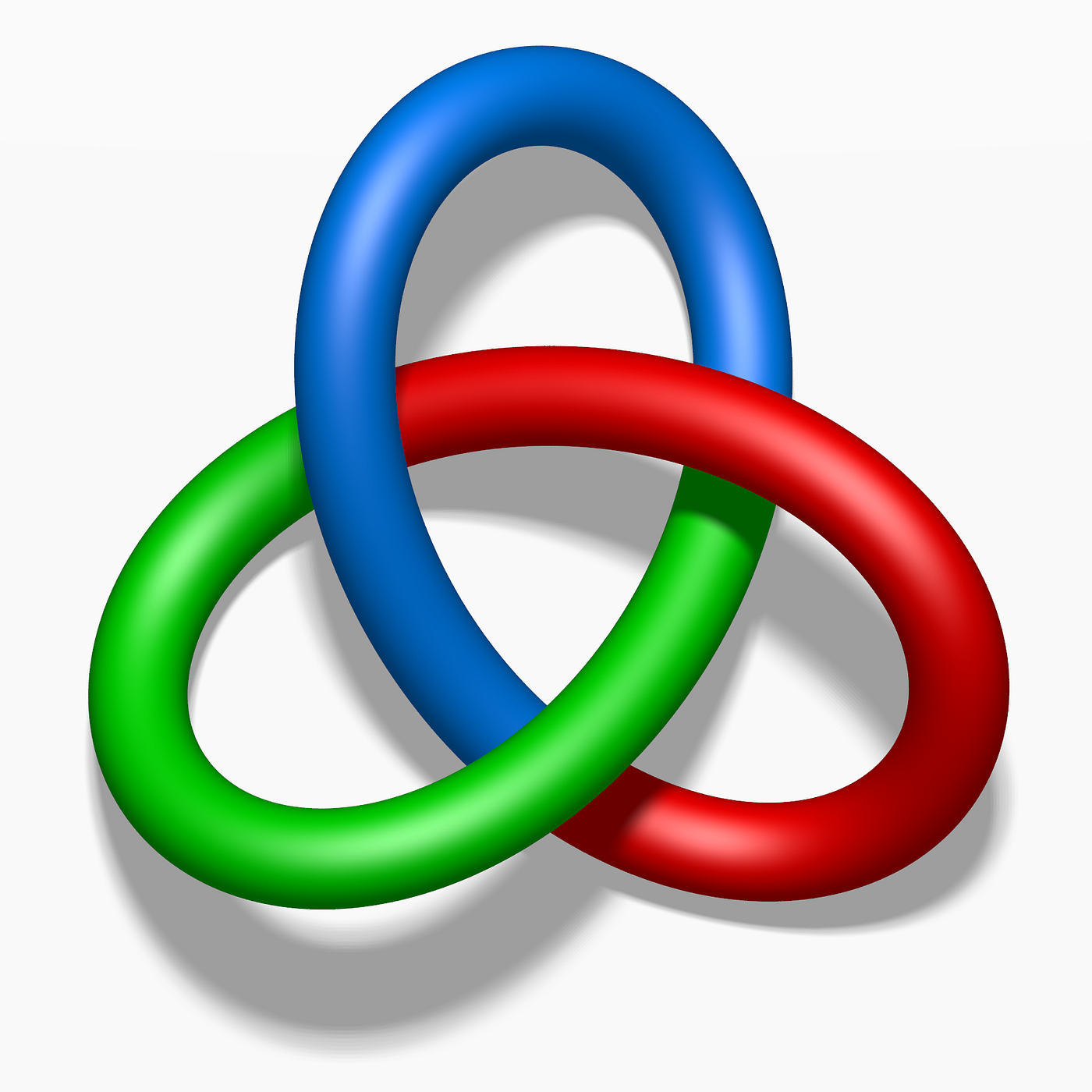
A tricolored trefoil knot. At each crossing, the three involved arcs have either all the same color or all different colors, so the diagram satisfies the tricolorability rule. Image by Jim.belk, via Wikimedia Commons, public domain.

Now compare this with the unknot. In its simplest diagram, the unknot is just one closed arc with no crossings. There is only one arc to color. Whatever color we choose, we have used only one color. But the rule demands at least two colors.

So the unknot is not tricolorable.

This is more than a coloring game. Tricolorability is preserved under Reidemeister moves. For example, Move I only adds or removes a small kink on a single arc. That kink does not force a genuinely new color choice; it is still the same strand locally folding over itself. Move II and Move III can also be checked locally: if the coloring rule is satisfied before the move, it can be satisfied after the move, and vice versa.

Therefore, if two diagrams are related by Reidemeister moves, either both are tricolorable or neither is.

The trefoil is tricolorable. The unknot is not.

This remains true even if the unknot is drawn with several crossings. The extra crossings create more arcs to color, but they do not create a genuine three-color structure. At each crossing, the three involved arcs must be either all the same color or all different colors. A failed coloring attempt usually gets stuck in the forbidden middle case: two arcs are forced to have the same color while the third has a different color.

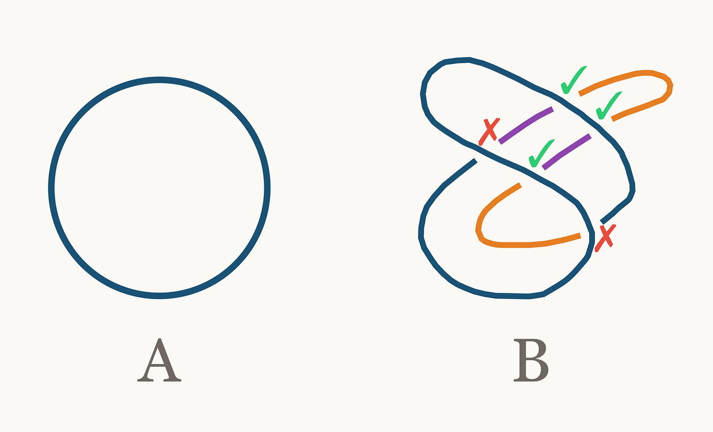
Two diagrams of the unknot. A is the standard circular diagram; B is a more complicated projection of the same knot. Neither is tricolorable: in B, a colouring attempt can satisfy some crossings but cannot be completed consistently.

Diagram B may look more complicated than diagram A, but it is still the same unknot. Its crossings belong to the drawing, not to a new knot. The coloring rules expose that fact: no matter how the colors are tried, every nontrivial attempt eventually fails.

Now the invariant has done its job.

So there cannot be a sequence of Reidemeister moves turning the trefoil into the unknot. The trefoil is not merely a badly drawn circle. It is genuinely knotted.

More powerful invariants were later developed, including polynomial invariants such as the Alexander polynomial and the Jones polynomial. These are much deeper than tricolorability, but the underlying principle is similar.

A knot invariant must not be fooled by the drawing.

And to prove that, it must survive Reidemeister’s three moves.

The Difficulty Beneath The Simplicity

There is a subtle irony in the Reidemeister theorem.

It is very easy to state. It is very easy to draw the three moves. It is tempting to think the theorem itself must be almost obvious.

It is not.

A rigorous proof has to address what kinds of knots and diagrams are being considered, how a three-dimensional knot is projected onto a plane, what kinds of crossings are allowed, and how to avoid pathological cases. In standard knot theory, one usually works with tame knots, meaning knots that behave well enough to be represented by ordinary diagrams.

There are also wild knots, whose behavior can be far more pathological. For these, ordinary knot diagrams may no longer capture the situation in the same clean way. The familiar world of crossings, projections, and finite diagrams assumes a certain regularity.

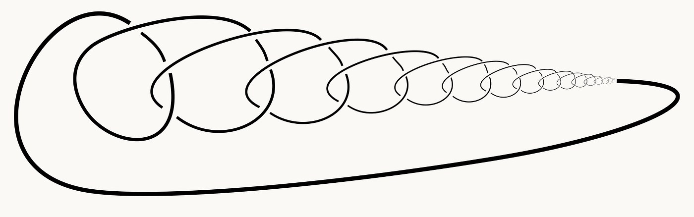
A depiction of a wild knot, whose infinitely accumulating structure lies outside the usual tame knot diagrams used in elementary knot theory. Image by Jkasd, via Wikimedia Commons, public domain.

This does not weaken Reidemeister’s theorem. It clarifies its domain.

Mathematics often works this way. A beautiful theorem may look simple only after the right definitions have been chosen. The simplicity is real, but it is not careless. It rests on precision.

That was part of Reidemeister’s achievement. He did not merely notice three convenient diagram tricks. He helped make knot theory exact.

When Knots Left The Page

For a long time, knot theory could have seemed like pure mathematical play.

A loop is tangled. Another loop is tangled. Are they the same? Can one become the other? Which properties remain unchanged?

But knots are not confined to chalkboards.

DNA molecules can become knotted and linked inside living cells. Enzymes that cut, pass, and reconnect strands of DNA are, in a physical sense, performing operations that knot theory helps describe. In chemistry, researchers have synthesized molecular knots, where the topology of the molecule affects its properties. In physics, knots and related structures appear in quantum field theory, statistical mechanics, and topological ideas about matter.

These applications do not replace the pure mathematics. They show why the pure mathematics had more reach than its first diagrams suggested.

A theory that began with closed loops on a page eventually became a way of thinking about structure, motion, and equivalence in the physical world.

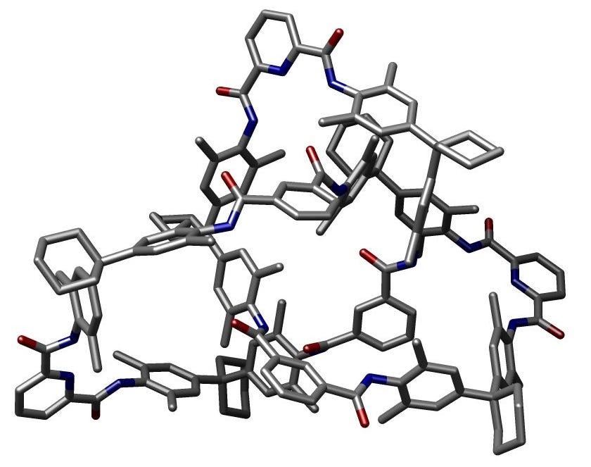
Crystal structure of a molecular trefoil knot reported by Vögtle and coworkers in Angewandte Chemie International Edition (2000, 39(9), pp. 1616–1618). Image generated from the published crystal structure data by M stone, via Wikimedia Commons, licensed under CC BY-SA 3.0.

The Grammar Of Tangled Things

A knot diagram can look like disorder.

A strand crosses over, then under, then over again. The eye follows the loop and gets lost. A small change in the drawing can make the whole object seem different.

Reidemeister showed that this disorder has syntax.

A twist may appear or disappear. Two crossings may be created or removed together. A strand may slide across a crossing. These three local moves do not solve every knot. They do not make all tangles simple. They do something more important.

They tell us when the drawing has changed but the knot has not.

That is the quiet beauty of the theorem. It does not deny complexity. It gives complexity a language.

A trefoil remains a trefoil, however it is drawn. The unknot remains the unknot, even when made to look unnecessarily tangled. And between two valid drawings of the same knot, somewhere, there is a finite path made of twists, passes, and slides.

The page may show a mess. But underneath the mess, there is order.