Reinforcement learning for AI engineers: How RL works, core trade-offs, and when not to use it

Reinforcement learning is a machine learning setup where an agent improves its decisions by interacting with an environment, experimenting, and receiving rewards or penalties that shape future behavior. The goal is to learn how to act over a sequence of steps so that long-term outcomes are good, not just a single prediction.

Why reinforcement learning matters

Reinforcement learning solves sequential decision problems with delayed feedback, which appear in control, recommendation, scheduling, and agentic AI. If you have already built supervised models, RL extends your toolbox from predicting to choosing actions that compound over time. This tutorial focuses on reinforcement learning and AI reinforcement learning as engineering disciplines rather than buzzwords.

By the end, you will be able to reason about mechanism, algorithm choice, trade-offs, and failure modes without relying on folklore. We will move from definitions to a small worked example, cover the main algorithm families, analyze production trade-offs, surface edge cases, and close with an honest when-not-to-use section.

What reinforcement learning is and what it is not

Reinforcement learning is the problem of learning a policy through interaction that maximizes expected cumulative reward. It is sequential decision-making under uncertainty, not generic learning from rewards in the abstract. The agent’s actions influence the future data it will see, so the objective is long-horizon control, not label matching.

A common formal lens is the Markov Decision Process with states, actions, transition dynamics, a reward function, and a discount factor. That lens is useful because it forces you to be explicit about what the agent observes, what it can do, and how outcomes are scored.

Reinforcement learning vs supervised, unsupervised, and self-supervised learning

Supervised learning maps inputs to labeled outputs; unsupervised learning finds structure; self-supervised learning creates proxy labels from data. Reinforcement learning differs because feedback is evaluative, possibly delayed, and depends on the agent’s own choices.

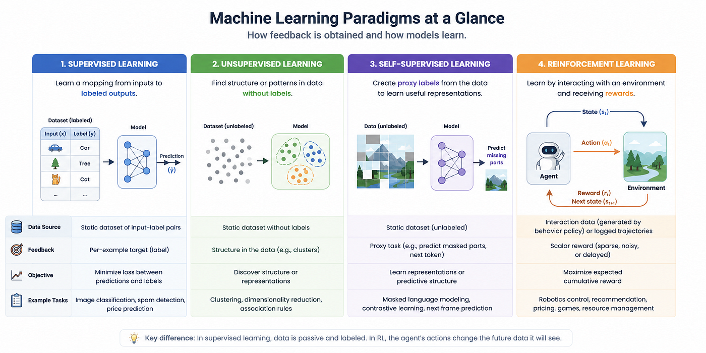
A compact comparison along practitioner-relevant axes:

Data source

• Supervised: static dataset of input-label pairs.
• Unsupervised or self-supervised: static dataset without human labels, or with proxy labels from the data.
• Reinforcement learning: interaction data generated by a behavior policy; may also learn from logged trajectories.

Feedback type

• Supervised: per-example target.
• Unsupervised or self-supervised: reconstruction, contrastive, or predictive surrogate.
• Reinforcement learning: scalar reward that can be sparse, noisy, or delayed.

Time horizon

• Supervised: one-shot.
• Unsupervised or self-supervised: one-shot or short context.
• Reinforcement learning: multi-step return.

Objective

• Supervised: minimize loss between predictions and labels.
• Unsupervised or self-supervised: learn representations or predictive structure.
• Reinforcement learning: maximize expected cumulative reward.

Deployment risk

• Supervised: behavior is passive at serve time.
• Reinforcement learning: actions change the world and future data; exploration carries operational risk.

Where confusion happens in practice:

• If actions do not affect future data, you may not need RL.
• Many ranking and ad-serving problems are contextual bandits rather than full RL.
• Search or planning with a known objective may beat learning a policy when a high-quality simulator or solver exists.

How reinforcement learning works

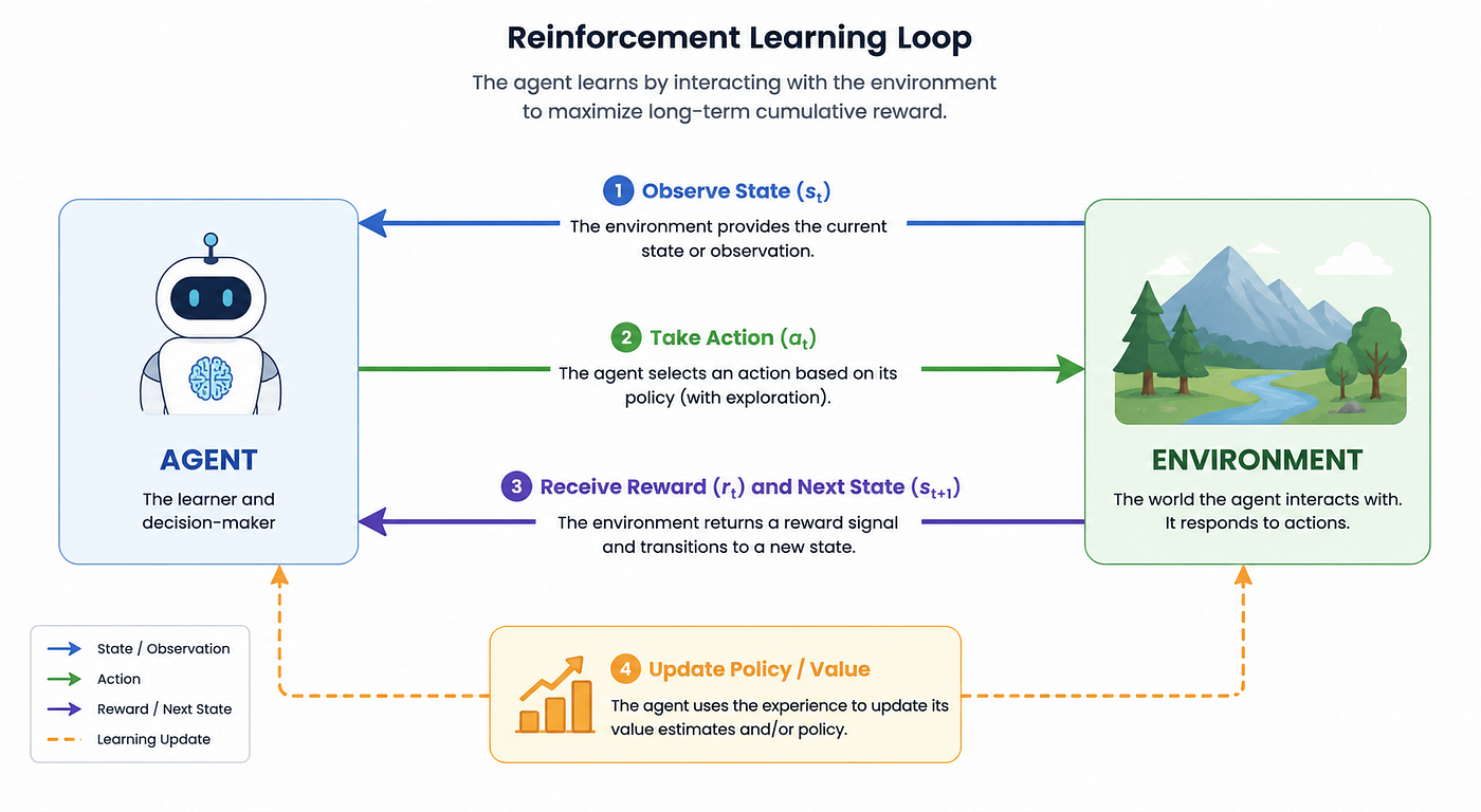
At a system level, reinforcement learning is a loop: observe a state, choose an action, transition to a new state, receive a reward, update what you believe and how you act, then repeat. The Markov Decision Process tuple is:

• States: what the agent needs to decide well.
• Actions: what the agent can do.
• Transition dynamics: how actions move you between states.
• Rewards: the scalar score per step.
• Discount factor: how much to weigh near-term vs far-future rewards.

Reinforcement learning introduces policy, value estimation, and exploration on top of prediction systems. Those pieces determine behavior, learning signals, and how you trade off trying new actions vs exploiting known good ones.

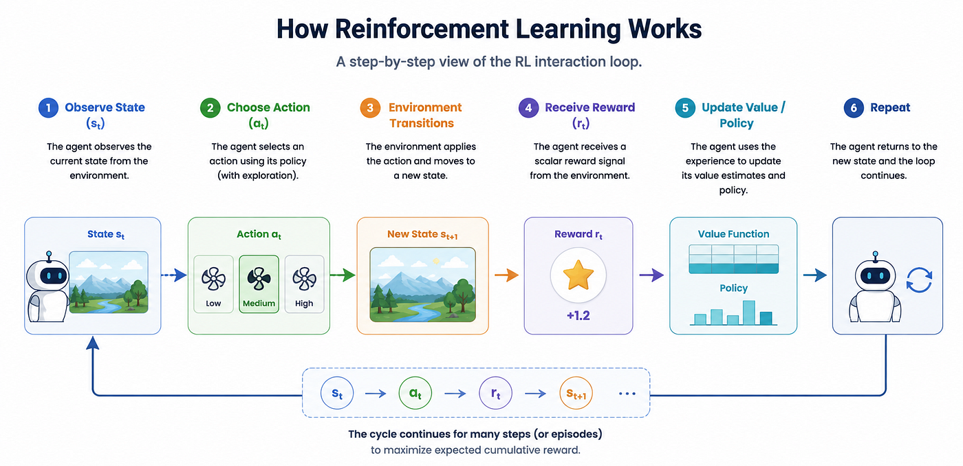
Agent, environment, state, action, and reward

• Agent: the learner and decision-maker that selects actions.
• Environment: everything the agent interacts with, including dynamics and reward generation.
• State: the information relevant for decision-making. It may be a compact vector, an embedding, or a discrete state identifier in tabular RL. Partial observability means the agent’s observation may not contain all relevant variables.
• Action: the control the agent applies, discrete or continuous.
• Reward: the scalar signal that scores outcomes per step or per episode.

Mapping to a real system:

• Robotics arm: state is joint angles and velocities; actions are torques; reward balances task success and energy.
• Recommender: state is user and context features; actions are items; reward is engagement or long-term retention.
• Cooling fan controller: state is temperature bucket; actions are fan settings; reward trades off comfort and energy.

Policy, value function, model, and return

• Policy: mapping from states to a distribution over actions; deterministic or stochastic.
• Reward signal: the immediate scalar feedback for a transition.
• Return: the discounted sum of future rewards. Discounting helps bound returns and down-weight distant, uncertain outcomes.
• Value function: expected return from a state under a policy. The action-value or Q-value is the expected return from a state-action pair.
• Model: a transition and reward predictor. Model-based reinforcement learning uses a model for planning; model-free RL learns values or policies directly.

Bellman intuition: a good state is one that leads to good future states. Value functions decompose return into immediate reward plus expected value of the next state.

Step-by-step learning loop

• Initialize behavior: pick a random or heuristic policy and value estimates.
• Observe state: read sensors or features that define the current decision point.
• Select action: apply the policy with exploration, for example epsilon-greedy or adding noise.
• Transition: environment returns next state and reward.
• Update: adjust value estimates and policy using the new experience.
• Continue: roll forward until an episode ends or indefinitely for continuing tasks.

Episodes reset the environment to stable starting conditions and simplify evaluation. The same loop underlies online learning, simulation training, and learning from logged trajectories with off-policy updates.

Worked example: reinforcement learning from scratch

A compact control task makes the mechanism concrete. We will implement tabular Q-learning with epsilon-greedy exploration. The problem is intentionally tiny so that the update rule and learned policy are easy to inspect before you consider Deep RL.

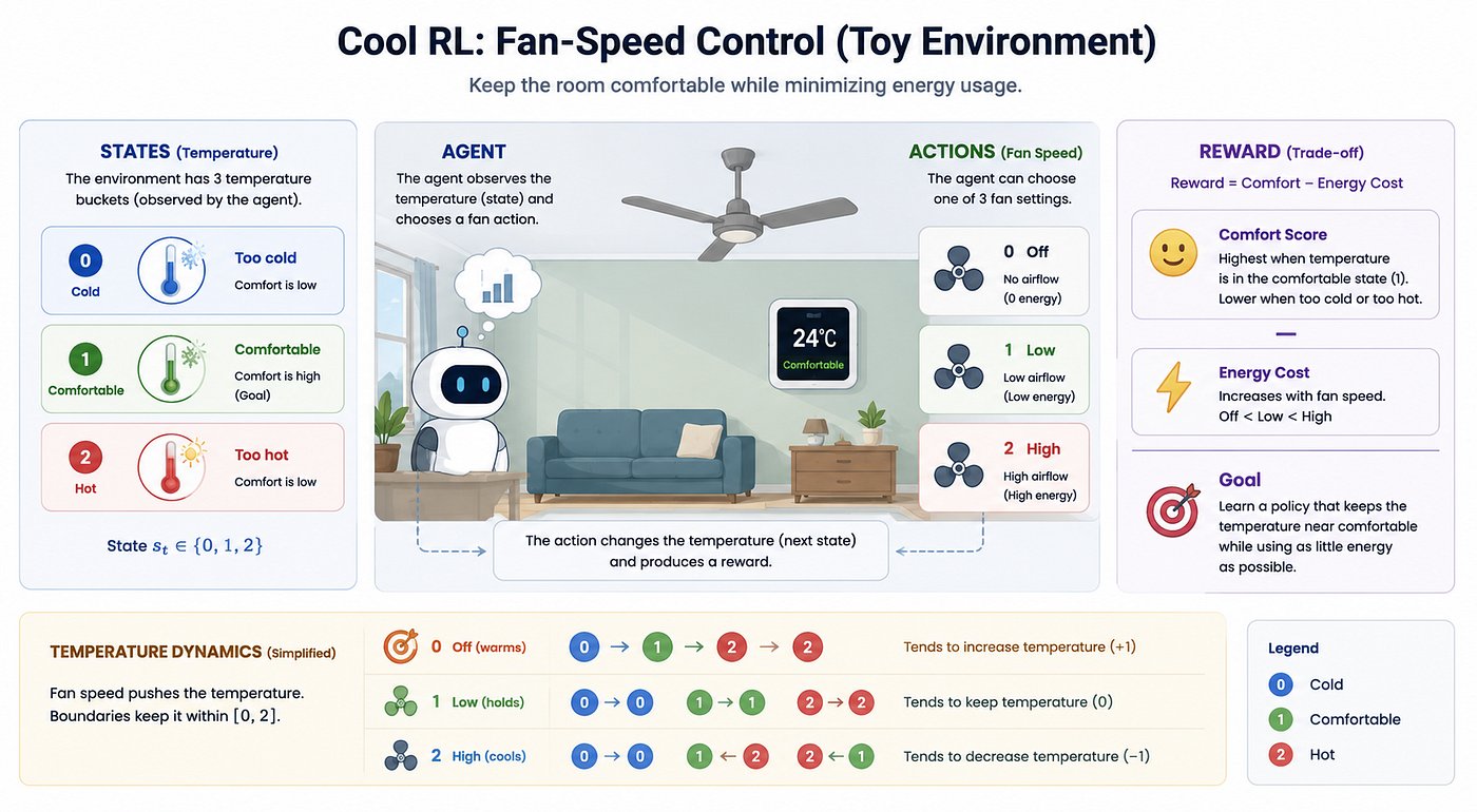
A “Cool RL” toy problem: fan-speed control

Environment design:

• State: three temperature buckets with integer identifiers 0=cold, 1=comfortable, 2=hot.
• Actions: three fan settings 0=off, 1=low, 2=high.
• Reward: comfort score minus energy usage. The agent should keep temperature near comfortable while minimizing energy.

Why this reward: optimizing comfort alone would always run the fan high; optimizing energy alone would keep the fan off. Combining them creates a nontrivial policy. Edge case to watch: a poorly weighted reward can teach the fan to save energy while letting the room stay hot, or to overcool aggressively and waste power.

Runnable Python snippet

Paste this into a Python file and run it. It implements tabular Q-learning with epsilon-greedy exploration and prints the learned policy and Q-table.

# cool_rl_q_learning.py
import random
import numpy as np

states = [0, 1, 2]          # 0=cold, 1=comfortable, 2=hot
actions = [0, 1, 2]         # 0=fan off, 1=low, 2=high
Q = np.zeros((len(states), len(actions)))

alpha = 0.2                 # learning rate
gamma = 0.9                 # discount factor
epsilon = 0.1               # exploration probability

def step(state, action):
    # simple temperature dynamics:
    # - fan off tends to warm the room (+1)
    # - fan low holds temperature (0)
    # - fan high cools the room (-1)
    next_state = max(0, min(2, state + (1 if action == 0 else 0 if action == 1 else -1)))
    # comfort is highest near state=1 (comfortable)
    comfort = {0: -1.0, 1: 2.0, 2: -1.0}
    # energy cost increases with fan speed
    energy = {0: 0.0, 1: 0.5, 2: 1.0}
    reward = comfort[next_state] - energy[action]
    return next_state, reward

# training
episodes = 5000
horizon = 10
for _ in range(episodes):
    s = random.choice(states)
    for _ in range(horizon):
        # epsilon-greedy action
        if random.random() < epsilon:
            a = random.choice(actions)
        else:
            a = int(np.argmax(Q[s]))
        s_next, r = step(s, a)
        # Q-learning update
        Q[s, a] += alpha * (r + gamma * np.max(Q[s_next]) - Q[s, a])
        s = s_next

labels = {0: "off", 1: "low", 2: "high"}
policy = {s: labels[int(np.argmax(Q[s]))] for s in states}
print("Learned policy:", policy)
print("Q-table:\n", Q.round(2))

One-line explanation of the update: move Q[s, a] toward immediate reward plus discounted value of the best next action.

What to expect:

• The policy typically converges to something like {0: “off”, 1: “low”, 2: “high”} or {0: “low”, 1: “low”, 2: “high”} depending on random seed and reward weights.
• The Q-table shows larger values for actions that move the system toward the comfortable state without overspending energy.

Try these modifications to see behavior shift:

• Increase the energy cost of action 2 to 1.5 and watch the policy rely more on action 1.
• Raise epsilon to 0.3 to explore more; convergence slows but avoids premature lock-in.
• Add stochasticity to dynamics, for example randomly flip next_state by plus or minus 1 with small probability, and observe the policy become more conservative.

Optional tracking with Weights & Biases Experiments:

• Install wandb, run wandb.login(), then log learning curves to compare settings side by side.

# Optional: track metrics with W&B
import wandb
wandb.login()
run = wandb.init(project="cool-rl", config=dict(alpha=alpha, gamma=gamma, epsilon=epsilon))
avg_return = 0.0
for ep in range(episodes):
    s = random.choice(states)
    G = 0.0
    for t in range(horizon):
        a = random.choice(actions) if random.random() < epsilon else int(np.argmax(Q[s]))
        s_next, r = step(s, a)
        Q[s, a] += alpha * (r + gamma * np.max(Q[s_next]) - Q[s, a])
        s = s_next
        G += r
    avg_return = 0.95 * avg_return + 0.05 * G
    wandb.log({"episode_return": G, "avg_return_ema": avg_return, "epsilon": epsilon, "episode": ep})
# Save the learned table as an artifact for reproducibility
np.save("q_table.npy", Q)
artifact = wandb.Artifact("cool-rl-qtable", type="policy")
artifact.add_file("q_table.npy")
wandb.log_artifact(artifact)
run.finish()

This adds a simple experiment record you can compare across hyperparameters, and it versions the learned Q-table as a W&B Artifact.

Algorithm families and when to use each

The main algorithm families differ by assumptions about your data and environment. Choose based on state size, action space, simulator access, safety constraints, and what you can log and evaluate.

Foundations:

• Dynamic programming: policy iteration and value iteration when the model is known exactly and state-action spaces are manageable.
• Monte Carlo methods: learn value from complete returns without bootstrapping.
• Temporal-difference learning: bootstrap from estimated values to update online and off-policy, bridging to modern methods.

When to use what:

• Tabular methods: small discrete state identifiers and actions; need transparency and easy debugging.
• Function approximation: states are large vectors or images; need generalization beyond visited states.
• Policy search and policy gradients: continuous action spaces or stochastic policies required by the task.
• Offline reinforcement learning: high-risk domains or scarce interaction budget with rich logged trajectories and careful evaluation.

Starter tools and prerequisites:

• Math: probability for expectations and conditional reasoning, linear algebra for function approximation, and dynamic programming concepts.
• Coding: Python, NumPy, and vectorization. For environments, use Gymnasium. For learning baselines, use Stable-Baselines3 or CleanRL. For distributed training and serving, consider RLlib. Use Weights & Biases Experiments or Sweeps to track runs and tune hyperparameters reproducibly.

Model-based vs model-free approaches

• Model-based reinforcement learning: plan using a known or learned transition and reward model. Advantages are sample efficiency and the ability to inspect plans. Risks are model bias and compounding error during long rollouts. Use when you have an accurate simulator, can learn one reliably, or when real-world samples are costly.
• Model-free RL: learn values or policies directly from experience. Advantages are simplicity and robustness to model misspecification. Costs are higher for sample needs and more trial-and-error. Use when interaction is cheap or when a reliable model is unavailable.
• Dynamic programming is the cleanest special case when the model is known and discrete.

Value-based, policy-based, actor-critic, and Deep RL

• Value-based reinforcement learning: estimate action values and act greedily, for example, Q-learning and its Deep RL variants. Often best for discrete actions.
• Policy-based: directly optimize a stochastic policy with gradients of expected return, for example, REINFORCE. Often best for continuous control or when stochasticity is required.
• Actor-critic: combine a policy (actor) with a value function (critic) to reduce variance and stabilize training, for example, A2C or PPO. Spans discrete and continuous actions.
• Deep RL: substitute neural networks for tables or linear functions to handle large or high-dimensional observations. Costs include instability, sensitivity to reward scaling and normalization, and higher compute and infrastructure demands.

The trade-offs that govern reinforcement learning in production

Reinforcement learning is shaped by unavoidable trade-offs rather than a single best algorithm. Exploration, sample use, compute, latency, determinism, and simulator fidelity interact with your domain, so state your choices explicitly.

Exploration vs exploitation

Exploration vs exploitation asks whether to try uncertain actions to learn more or to keep using actions that already look good. RL cares more than supervised learning because the agent’s actions determine future data.

Common strategies:

• Epsilon-greedy for simple discrete problems.
• Optimistic initialization to encourage early exploration.
• Entropy bonuses in policy gradients to maintain stochasticity.
• Upper-confidence approaches that bias toward actions with higher uncertainty.

Edge cases:

• User-facing systems, robots, and finance often make naive exploration unsafe or expensive; consider simulated pre-training, risk constraints, or conservative policies.

Accuracy vs latency, cost vs throughput, and flexibility vs determinism

• Accuracy vs latency: larger networks or deeper planners can improve decision quality but raise inference time. For real-time control, cap model size and precompute lookups or policies. For batch recommenders, accept slower inference if it improves long-term objectives.
• Cost vs throughput: more rollouts, richer simulators, and larger replay buffers often improve performance but increase compute and wall-clock. Use parallel simulation and prioritize sample reuse with off-policy methods when budgets are tight.
• Flexibility vs determinism: stochastic policies adapt to non-stationary environments and support exploration; deterministic policies are easier to audit and safer in regulated settings. Consider mixed strategies, for example stochastic online with deterministic fallbacks.
• Simulator fidelity vs reality gap: high-fidelity simulators improve offline training but widen the gap if they omit real-world noise or delays. Domain randomization and targeted real-world calibration reduce surprises.

Failure modes, edge cases, and evaluation

Many RL systems appear to work well in training but fail to achieve the true objective in deployment. The common pitfalls are not rare edge cases but everyday engineering issues: reward hacking, sparse rewards, non-stationarity, partial observability, delayed consequences, and sim-to-real mismatch.

Evaluation is hard because counterfactual outcomes are missing. Online A/B tests are risky and expensive, while offline metrics can be misleading under a distribution shift. Make evaluation plans a first-class artifact of the project.

Reward design, sparse feedback, and credit assignment

A reward is a proxy for the real goal. If the proxy is wrong, the agent will exploit it. Sparse feedback and long delays make credit assignment difficult because useful signals arrive far from the actions that caused them.

Concrete example patterns:

• Recommenders that over-optimize short clicks at the expense of long-term satisfaction.
• Control systems that minimize energy by avoiding work while missing service-level targets.

Mitigations:

• Shape rewards carefully with explicit constraints for safety and service levels.
• Add penalties for anticipated pathological behaviors.
• Use imitation learning or human feedback to bootstrap before outcome-based optimization.
• Redesign the environment to provide intermediate feedback or curriculum stages.

Offline vs online RL, off-policy evaluation, and identifiers

• Online reinforcement learning: learns while acting and collecting new experiences.
• Offline reinforcement learning: learns from fixed logged data without additional interaction.

Offline reinforcement learning is attractive when exploration is unsafe, but it fails when the logged policy does not cover the important states or actions. Instrumentation matters: log action probabilities when possible, timestamps, rewards, trajectory boundaries, and a stable episode or user identifier to reconstruct sessions.

Off-policy evaluation aims to estimate the performance of a new policy using old data. It is brittle under distribution shift and poor coverage. Improve reliability through careful logging, sanity-check baselines, and conservative policy improvements that stay close to the behavior policy.

Where AI reinforcement learning is actually useful

Use reinforcement learning when decisions compound over time and labels alone do not capture what you care about.

Representative use cases and why they are reinforcement learning problems:

• Robotics and industrial control: the controller’s actions affect future system states, and success is a long-horizon property.
• Recommenders and feeds: each recommendation changes the user's state and future opportunities; short-term clicks do not fully reflect long-term value.
• Bidding and pricing: actions affect competitor responses and user demand trajectories.
• Scheduling and resource management: allocations today shape tomorrow’s queues and latencies.
• Finance and trading: actions change the portfolio and risk over time.
• HVAC and fan control: actions influence future temperature and energy spent, not just the next reading.

Modern AI assistants and reinforcement learning:

• Large language model assistants have used reinforcement learning from human feedback by training a reward model on preference data and optimizing a policy using algorithms such as PPO. The appeal is that outcome-based optimization can better align behavior with user preferences than imitation alone, but it inherits the usual RL risks of reward misspecification and evaluator quality.

Reinforcement learning for agentic AI and Agent Lightning-style systems

Reinforcement learning is re-emerging in agentic AI because tool use, planning, and multi-step task completion yield delayed rewards that supervised fine-tuning cannot capture. RL can optimize for end-to-end outcomes, such as successful job completion, rather than per-step imitation.

When reinforcement learning helps:

• The task spans many steps with branching choices and tool calls.
• Success is measured at the end with a scalar metric, for example success or cost.
• You can simulate tasks or gather logged trajectories at scale.

When reinforcement learning is overkill:

• High-quality demonstrations already match the desired behavior.
• Tools and APIs change rapidly, creating non-stationarity faster than the agent can learn.
• Evaluators are noisy or biased, creating reward hacking risk.

Edge cases unique to agentic systems:

• Non-stationary tools and flaky evaluators produce drifting rewards.
• Sparse terminal rewards make credit assignment hard; dense proxies or subgoal shaping can help.
• Long-horizon credit assignment often benefits from curriculum design and hierarchical policies.

When not to use reinforcement learning

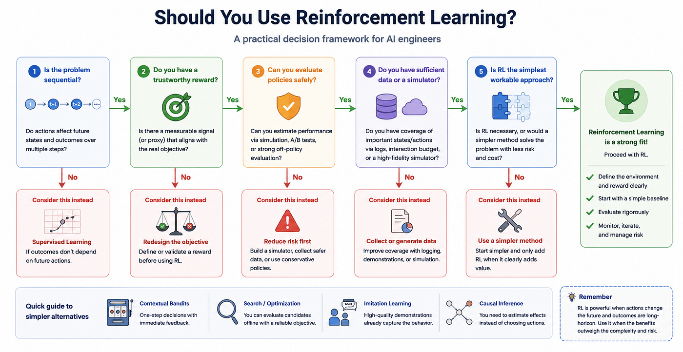
Do not start with reinforcement learning when:

• A supervised objective already matches the business goal and does not depend on future actions.
• You cannot define a trustworthy reward that aligns with the real objective.
• Exploration is unsafe or illegal, and you lack a high-coverage logged dataset or simulator.
• The environment is mostly one-shot or static, so actions do not influence future data.

Simpler alternatives by problem shape:

• Supervised learning for direct predictions that drive rule-based actions.
• Contextual bandits for one-step action selection with per-decision feedback.
• Search or optimization when you can evaluate candidates offline with a reliable objective.
• Imitation learning when demonstrations are abundant and sufficient.
• Causal inference when you need counterfactual estimation rather than control.

Operational note: adopting reinforcement learning commits you to data collection, evaluation, and risk-management workflows, not just to a new algorithm.

A practitioner’s litmus test

Use this quick decision checklist before reaching for RL:

• Is the problem truly sequential, where actions affect future data and outcomes?
• Is there a measurable reward or proxy you can trust, with a plan to refine it safely?
• Can you evaluate policies without unacceptable risk, via simulation, A/B tests, or strong off-policy evaluation?
• Do you have sufficient coverage, logged trajectories, or a simulator to learn from?
• What is the simplest workable method that preserves the problem’s structure?

Start small, as in the Cool RL example, to validate mechanics and incentives. The same loop scales to production with different state spaces, models, and constraints, but the engineering principles and trade-offs do not change.