TF-IDF (Term Frequency-Inverse Document Frequency) Explained

TF-IDF is essentially word counting, but with additional weighting based on how informative each word is.(Photo by Ahmadreza Rezaie on Unsplash)

I once created a project for BBC News using TF-IDF to predict the engagement time of news articles. The idea was to build a benchmark that editorial teams could use to optimise articles and make better placement decisions.

Machine learning algorithms work with numbers, not paragraphs. Before a model can learn from text, we need a way to convert language into numerical features. TF-IDF is essentially a smarter version of word count.

The Problem With Raw Text

One common first step in natural language processing (NLP) is converting text into structured numerical features.

For example, suppose we want to predict how often a student is late to school each week based on a short written statement.

Here is the first student:

“I go to school by bus. I go home by bus.” (late: 1 time per week)

We can transform this sentence into numerical features simply by counting words:

This becomes one row in a dataset.

Now imagine collecting data from another student:

“I go to school on foot. I go home on foot.” (late: 3 times per week)

Even from this tiny example, patterns immediately appear.

The words “by” and “bus” seem associated with fewer late arrivals, while “on” and “foot” seem associated with more lateness.

That signal is enough for a machine learning model to begin learning relationships between language and outcomes.

This simple counting process is known as term frequency (TF).

Why Word Count Alone Is Not Enough

If we only use raw word counts, we implicitly assume every word is equally important. But clearly that is not true.

Words like “I”, “go”, and “school” appear in almost every sentence. They do not really tell us anything useful about whether someone will be late.

In NLP, extremely common words are often less informative precisely because they appear everywhere.

This is where inverse document frequency (IDF) comes in.

Instead of asking:

“How often does this word appear in this document?”

We also ask:

“How often does this word appear across all documents?”

If a word appears in nearly every document, it probably is not very useful for distinguishing between them.

Inverse Document Frequency

Let us combine both students’ sentences into a small corpus.

Now we count how many documents each word appears in.

Notice how words like “I” and “go” appear very frequently across the corpus. That suggests they carry less unique information.

To reduce the importance of overly common words, we assign lower weights to terms with high document frequency.

For intuition, we can simplify this as:

So:

The idea is that:

Common words receive lower importance. Rare and distinctive words receive higher importance.

Putting It Together: TF-IDF

Finally, we combine both ideas together:

TF-IDF = TF × IDF

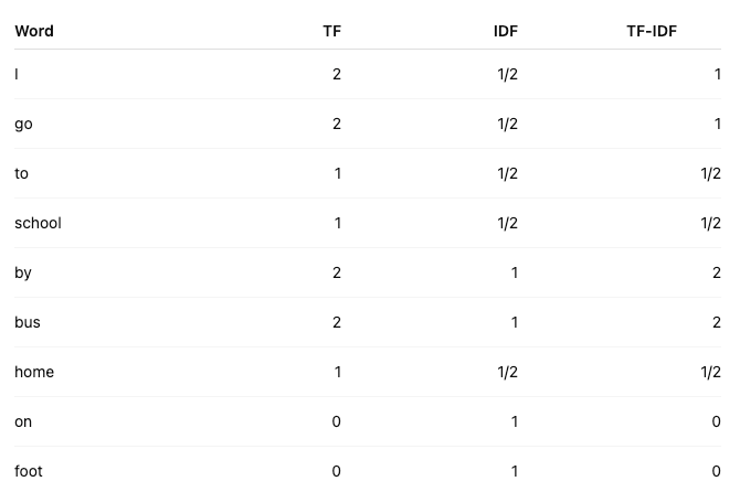
For the first student:

• “bus” appears frequently in the sentence
• but not excessively across all documents

So it receives a relatively strong weight.

Meanwhile, words like “I” and “go” are heavily down-weighted because they appear everywhere.

The final TF-IDF vectors look something like this:

How scikit-learn’s TF-IDF Is Different From the Simple Formula

The actual IDF formula used by scikit-learn is approximately:

Where:

• n = total number of documents
• df(t) = number of documents containing term t

1. Logarithmic Scaling

The logarithm prevents extremely rare words from receiving absurdly large weights.

Imagine a word that appears in only one article out of one million. If we simply used division, its importance score could explode to an unrealistic level.

The logarithm compresses the scale so that rare words still receive higher importance, but not excessively so.

This makes the model much more stable.

2. Smoothing

Notice the extra “+1” terms in the formula. These are used for smoothing.

Without smoothing, extremely rare terms can create numerical edge cases. Adding 1 avoids mathematical edge cases and keeps the computation numerically stable.

3. Vector Normalisation

After computing TF-IDF scores, scikit-learn also normalises the resulting vectors.

This means long documents do not automatically dominate simply because they contain more words.

For example, a 5,000-word article would naturally have much larger raw counts than a 200-word article. Normalisation rescales the vectors so documents become more comparable regardless of length.

This is an important detail because otherwise models might accidentally learn “article length” instead of meaningful language patterns.

4. Tokenisation and Preprocessing

Scikit-learn also performs preprocessing automatically.

By default:

• text is lowercased
• punctuation is generally excluded during tokenisation
• words are tokenised
• single-character words like “I” are removed

What Machine Learning Algorithms Do We Usually Use With TF-IDF?

After transforming text using TF-IDF, we end up with a large numerical table.

These transformed representations are usually called:

• feature vectors
• TF-IDF vectors
• document vectors
• sparse vectors

The word “vector” simply means a list of numbers representing a document.

For example, an article might become something like:

[0.0, 0.24, 0.0, 0.81, 0.13, ...]

Each position corresponds to a word in the vocabulary, and each value represents that word’s TF-IDF weight.

Once text has been converted into vectors, we can feed those vectors into standard machine learning algorithms.

Some of the most common algorithms used with TF-IDF include:

• Classification: Logistic Regression, Naive Bayes, Linear SVM
• Regression: Ridge Regression, Linear Regression
• Clustering: K-Means
• Recommendation/Search: Cosine Similarity

One interesting thing about TF-IDF is that it often works surprisingly well with relatively simple linear models. That is because TF-IDF already does much of the heavy lifting by extracting meaningful signals from language.

For my BBC News engagement prediction project, I used Ridge Regression, which is Linear Regression with an additional penalty term that discourages overly large coefficients.

In NLP problems, the number of features can become enormous. Even a modest news dataset might produce tens of thousands of unique words.

That means many features are sparse (the vast majority of entries are zero), many words are correlated, some words appear only rarely, and the model can easily overfit.

Ridge Regression helps stabilise the model by shrinking coefficients toward smaller values. This is particularly useful for text data because language naturally contains noise, redundancy, and accidental correlations.

For example, maybe one article containing the word “earthquake” happened to receive unusually high engagement. A plain linear model might assign an excessively large weight to that word based on limited examples.

Ridge Regression reduces this problem by shrinking the coefficients toward smaller values. It tends to perform especially well for high-dimensional data, sparse feature spaces, and datasets with many correlated features.

Common TF-IDF Hyperparameters to Tune

1. max_features controls the maximum number of words or phrases kept in the vocabulary. For example, max_features=5000 means we only keep the top 5,000 terms. This is useful because real text data can contain thousands or even millions of unique words. Many of them may be rare typos, names, or one-off phrases that add noise rather than useful signal.
2. min_df removes words that appear in too few documents. For example, min_df=5 means a word must appear in at least 5 documents to be included. This helps remove very rare words that may not generalise well.
3. max_df removes words that appear in too many documents. For example, max_df=0.9 means we ignore words that appear in more than 90% of documents. This is useful for filtering out extremely common words. In a news dataset, words like “said”, “people”, or “news” may appear so often that they do not help distinguish one article from another.
4. ngram_range controls whether we only use individual words or also include short phrases. For example, ngram_range=(1, 2) means we include both single words and two-word phrases. This can be very powerful because sometimes meaning lives in phrases, not individual words. The word “prime” alone may not say much, and “minister” alone may not say much, but “prime minister” is clearly meaningful.
5. stop_words removes common words such as “the”, “and”, “is”, and “in”. For English text, we can use stop_words=”english”. This is not always automatically better, though. Sometimes common words still carry useful signals depending on the task, so it is worth testing.
6. sublinear_tf changes how term frequency is counted. Instead of allowing repeated words to keep increasing linearly, it dampens the effect of repetition using a logarithmic scale. It applies a logarithm to the term frequency (TF) part: TF = 1 + log(tf) For example, if a word appears 20 times in an article, that does not necessarily mean it is 20 times more important than a word that appears once. sublinear_tf=True helps reduce that problem.
7. norm controls how the final TF-IDF vectors are normalised. The default is norm="l2". Normalisation helps make documents more comparable, especially when some articles are much longer than others.

The important point is that TF-IDF tuning is about controlling the vocabulary and the weight of each term. We are trying to keep enough words to capture meaning, but not so many that the model gets distracted by noise.

Python Implementation

from sklearn.feature_extraction.text import TfidfVectorizer
from sklearn.linear_model import Ridge
from sklearn.model_selection import GridSearchCV, train_test_split
from sklearn.pipeline import Pipeline
from sklearn.metrics import mean_absolute_error, mean_squared_error, r2_score

# In a real project, this would contain thousands of news articles.
documents = [
    "The government announced a new education policy today.",
    "The football team won the final after a dramatic penalty shootout.",
    "Scientists discovered a new method for detecting early disease.",
    "Markets fell sharply after concerns about inflation increased.",
    "A new film release has received strong reviews from critics."
]

# Average engagement time per article (in seconds).
engagement_time = [42, 65, 58, 37, 49]

# Split the data into training and testing sets.
X_train, X_test, y_train, y_test = train_test_split(
    documents,
    engagement_time,
    test_size=0.2,
    random_state=42
)

# Create a pipeline.
# Step 1: Convert text into TF-IDF vectors.
# Step 2: Feed the vectors into a Ridge Regression model.
pipeline = Pipeline([
    ("tfidf", TfidfVectorizer()),
    ("model", Ridge())
])

# Hyperparameters to test during tuning.
param_grid = {
    # Maximum vocabulary size. Keeps only the most important terms.
    "tfidf__max_features": [1000, 3000, 5000],

    # Ignore words appearing in too few documents.
    "tfidf__min_df": [1, 2],

    # Ignore overly common words.
    "tfidf__max_df": [0.8, 0.9, 1.0],

    # Use single words only OR single words + two-word phrases.
    "tfidf__ngram_range": [(1, 1), (1, 2)],

    # Optionally remove English stop words.
    "tfidf__stop_words": [None, "english"],

    # Apply logarithmic scaling to term frequency.
    "tfidf__sublinear_tf": [False, True],

    # Ridge regularisation strength.
    "model__alpha": [0.1, 1.0, 10.0, 100.0]
}

# GridSearchCV performs cross-validation
# and searches for the best parameter combination.
grid_search = GridSearchCV(
    estimator=pipeline,
    param_grid=param_grid,
    scoring="neg_mean_absolute_error",
    cv=2,
    n_jobs=-1
)

# Train all combinations.
grid_search.fit(X_train, y_train)

# Retrieve the best-performing pipeline.
best_model = grid_search.best_estimator_

# Generate predictions on unseen test data.
predictions = best_model.predict(X_test)

print("Best parameters:")
print(grid_search.best_params_)

print("\nModel performance:")
print("MAE:", mean_absolute_error(y_test, predictions))
print("MSE:", mean_squared_error(y_test, predictions))
print("R²:", r2_score(y_test, predictions))