Permutation Feature Importance from Scratch

Understanding the importance of permutations in the field of explainable AI

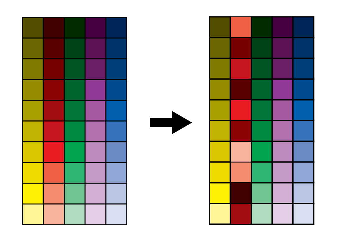
(source: author)

If you look under the hood of the most advanced XAI methods, you will find permutations. SHAP, LIME, PDPs & ICE Plots, ALEs and Friedman's H-stat all rely on them. This is why understanding permutations and their limitations is so important to the field. So, let’s start with the simplest XAI method — permutation feature importance (PFI).

To gain a deep understanding of this approach we will:

• Calculate PFI from scratch using Python.
• Explain the choices behind the method including why we permute, repeat and which metric to use.
• Discuss the limitations of permutations.

You can find the full project on GitHub.

You may also enjoy this video on the topic. And, if you want to learn more, check out my course — XAI with Python. You can get free access if you sign up to my newsletter.

[embed]

Why PFI?

Feature importance scores are a collection of methods that all aim to tell us one thing — which features are most important to a model’s predictions in general. They include counting the number of splits in the tree or the mean effect plot. Amongst all these, permutation feature importance is the most popular. This is due to two reasons.

Firstly, as we will see, it has an intuitive calculation. This makes it easy to explain to a non-technical audience. Secondly, it is model agnostic. In the case of PFI, permuting means we rearrange or randomly shuffle the values of model features. We then summarise changes in the model predictions using some metric. In other words, the process is always the same regardless of what model you use. We will see this when calculating the scores.

PFI from scratch

Before calculating PFI, we need a model. We will use XGBoost (line 8). You may notice, there is no package to calculate PFI. As mentioned, we will calculate the scores from scratch.

import matplotlib.pyplot as plt
import seaborn as sns

import numpy as np
import pandas as pd

import xgboost as xgb
from sklearn.metrics import accuracy_score,confusion_matrix

To explain how this method works, we will be using the credit score dataset. You can see a snapshot in Figure 1. It contains 84 features for 1000 customers based on their transactions and financial position. We use this dataset to estimate a customer’s credit risk which is given by CREDIT_SCORE. You can find the full description on Kaggle.

Figure 1: snapshot of credit score dataset (source: author) (licence: CC0: Public Domain)

We load our data (line 2). We select 5 features including a customer's total income in the last 12 months (INCOME) and total existing debt (DEBT). We also need to create some dummy variables from CAT_GAMBLING which is a categorical feature with 3 groups (lines 9–11). Finally, we select our target variable (line 14).

# Load dataset and add squared term
credit_score = pd.read_csv("../../data/credit_score.csv")

# Select features
features = ['INCOME','DEBT','R_EXPENDITURE','R_ENTERTAINMENT','CAT_GAMBLING']
X = credit_score[features].copy()

# One-hot encoding
X['GAMBLING_LOW'] = X['CAT_GAMBLING'].apply(lambda x: 1 if x == 'Low' else 0)
X['GAMBLING_HIGH']  = X['CAT_GAMBLING'].apply(lambda x: 1 if x == 'High' else 0)
X.drop(columns=['CAT_GAMBLING'], inplace=True)

# Target variable
y = credit_score['CREDIT_SCORE']

We train our XGBoost model (lines 2–3). To avoid overfitting, we have set the max depth to 3. Keep in mind, that when you are applying model agnostic methods, you should always follow best practices (e.g. train test split). The better your model the more reliable your interpretations will be.

# Train model
model = xgb.XGBRegressor(objective="reg:squarederror", max_depth=3, n_estimators=100) 
model.fit(X, y)

Evaluating the model

We can visualise the performance of the model using a residual plot. We get the model predictions for all 1000 customers (line 2) and plot these against their actual credit score (line 7). Remember, the red line (line 8) gives the line of perfect predictions. We can see the result in Figure 2. By comparing the scatter points to this line we can understand how well the model is doing.

# Get predictions
y_pred = model.predict(X)

# Model evaluation
fig, ax = plt.subplots(nrows=1, ncols=1,figsize=(8,8))

plt.scatter(y,y_pred)
ax.plot([y.min(), y.max()], [y.min(), y.max()], color='tab:red')

plt.ylabel('Predicted',size=20)
plt.xlabel('Actual',size=20)

Figure 2: residual plot of actual vs predicted credit score for the XGBoost model (source: author)

It is difficult to use this visualisation to compare the performance of multiple models. So, we need a way of summarising all the residuals. For regression, a common metric is the coefficient of determination or R-squared value. The higher the R-squared value the more accurate the predictions and perfect predictions would give an R-squared value of 1.

With XGBoost, this metric is used by default by the score function (line 2). Using the code, we get an R-squared value of 0.93. For PFI, we take this as our baseline score — the score when no feature has been permuted. We can compare changes to this baseline when we start permuting features.

# Calculate performance metric
baseline_score = model.score(X, y)

baseline_score

Permuting a feature

Permuting a feature means we shuffle the values of that feature. For PFI, we do this one feature at a time. As we will discuss later, only the values for the given feature must be used. We saw an abstract representation in the article’s cover image. There you can see how the values from the red feature have been randomly shuffled.

Let’s do this for a real feature. We make a copy of the feature matrix (line 1) and permute the income feature (line 2). Using the model we trained on the original dataset we make predictions on the dataset with this permuted feature (line 5). Using a residual plot, we can visualise the accuracy of these predictions in the same way as before. Looking at Figure 3, we can see it is a mess! This tells us that INCOME is being used by the model to make predictions.

X_perm = X.copy()
X_perm['INCOME']= np.random.permutation(X_perm['INCOME'])

# Get predictions
y_pred = model.predict(X_perm)

Figure 3: residual plot when INCOME is permuted (source: author)

This is the core idea behind PFI. The model is using the relationship between INCOME and credit score to make predictions. When we permute income we break this relationship and so the model makes worse predictions. Again, it is difficult to make an objective judgement on how much worse by using a visualisation.

Instead, we can calculate the R-squared value for the permuted predictions (line 2). This gives us a value of -3.26. The importance score is the baseline score less this permuted score (line 5). We get a value of 4.19 = 0.93 — (-4.19). This is our measure of feature importance — the decrease in R-squared when the feature is permuted.

# calculate performance metric on permuted data
permuted_score = model.score(X_perm, y)

importance_score = baseline_score - permuted_score
importance_score

Putting it all together

Using the get_perm_importance function, we can do the above calculation for multiple features. We pass in our model, feature matrix, target variable and list of features. You may also notice the n parameter. By default, we will repeat the calculation 10 times and take the average as our final importance score (line 28). We discuss the logic behind this later.

def get_perm_importance(model, X, y, features, n=10):

    """
    Calculate permutation importance score for each feature
    """

    # Calculate baseline score (without permuting any feature)
    baseline_score = model.score(X, y)

    importance_scores = {}

    # Loop over each feature
    for feature in features:

        X_perm = X.copy()
        sum_score = 0

        # Repeat n times to get average importance score
        for i in range(n):

            # Calculate score when given feature is permuted
            X_perm[feature]= np.random.permutation(X_perm[feature])
            permuted_score = model.score(X_perm, y)

            sum_score += permuted_score

        # Calculate decrease in score
        importance_score = baseline_score - sum_score/n
        importance_scores[feature] = importance_score

    return importance_scores

We apply this function to our XGBoost model and calculate the scores for all the features in the X matrix (line 2). We sort the scores from highest to lowest (lines 5–6) and visualise them using a bar plot (lines 8–10). In Figure 4, you can see DEBT and INCOME are the most important features.

# Calculate permutation feature importance
importance_scores = get_perm_importance(model, X, y, X.columns,n=10)

# Display the importance scores using a horizontal bar plot
sorted_importance_scores = sorted(importance_scores.items(), key=lambda x: x[1])
features, scores = zip(*sorted_importance_scores)

plt.subplots(figsize=(8,4))
plt.barh(features, scores)
plt.xlabel('Permutation Importance')

Figure 4: permutation feature importance scores (source: author)

Logic behind PFI

Why permute?

You may be tempted to replace a feature’s value with any randomly sampled values. However, we permute a feature, as it is important to sample from the same distribution as the original values for that feature. This ensures that the permuted feature values are realistic and representative of the variability observed in the actual dataset. If we sample from a different distribution, we may introduce unrealistic scenarios that could lead to misleading importance scores.

Take the INCOME feature. Instead of permuting, suppose we replaced its values with smaller-than-average income values or even negative values. This may lead the model to make predictions that are consistent with low-income customers. In other words, it may only predict low credit scores and skew the importance score for this feature.

There are a few ways to permute features:

• For LIME, we sample from a normal distribution with the same mean and standard deviation as the feature.
• For PDPs, we sample from the entire range of the feature.
• For ALEs, we sample from a small interval around a feature value.

In all cases, we will not sample values that are vastly different from the original feature values.

Why repeat?

Trying the permutation code above that calculated the importance score for income, you will get a different value that is not 4.19. This is because permutation is a random process and there will be variability in the values calculated. This is why we repeat the permutation process and take the average of the scores. The result is a more reliable estimation of feature importance.

Why R-squared?

There is nothing special about R-squared. It is just a common metric. We could have used any metric for evaluating regression models such as MSE. For classification problems, it is common to use accuracy or AUC but you can also use precision or recall. You should use whatever metric or collection of metrics that make sense for your application and audience. If you want to change the metric you will have to update lines 8 and 23 in the get_perm_importance function.

The limitations of permutations

PFI is straightforward and useful to gain an overview of how your model works. It does however have its limitations. PFI only provides a simple global interpretation, ignores interactions and cannot be used for causal inference. Yet, the most significant limitation is the assumption that features are independent. This can lead to an unreliable estimate of a feature’s importance.

Assumption of independence

If two features are associated or correlated then the value of one feature will change when we change the value of the other. Yet, with PFI we only permute/change the values of one feature at a time. In other words, we are assuming that features are not associated — that they are independent. This assumption can give us misleading feature importance scores in two ways.

Firstly, a model could compensate for the absence of one feature by relying on its correlated counterpart. Suppose we included an additional measure of income in our model, INCOME_6. This is a person’s income over the last 6 months. In Figure 5, we can see this to be highly correlated with INCOME — income over the last 12 months.

We can expect that both features have similar relationships with the target variable. So, to an extent, if we permuted INCOME_6 the model could still make accurate predictions using INCOME and visa versa. The result could be low scores, for both features, that do not capture their true importance.

Figure 5: scatterplot of income in last 12 months vs last 6 months. The red line gives the values when the two income features are equal (source: author)

Secondly, we could end up with feature value pairs that the model was not trained on leading to unreliable predictions. Take the same features INCOME and INCOME_6. After permuting the latter, we would have cases where a customer had more income in the last 6 months than in the last 12 months. In Figure 5, we would create instances below the red line. We can see that is not possible and we cannot know what effect it will have on model predictions.

I have correlated features, now what?

All permutation-based approaches are impacted in the same way. In fact, the only model agnostic method that avoids this assumption is ALEs. So, if you have multicollinearity, the first step is to try and remove the highly correlated features. However, these features may still improve model performance even though they are highly correlated. In this case, do not avoid the other methods.

The effects mentioned above will not necessarily have a large impact on the results of model agnostic methods. They can still provide useful insight into your model. You just need to use them with an increased level of caution:

• Use more than one XAI approach. You can be more certain about a conclusion if they all agree.
• Use data exploration. Find creative ways of aggregating the data so you can see the same relationships in the raw data.
• Incorporate domain knowledge. If a relationship aligns with what was already expected you can be more certain about the interpretation.

With this understanding, we can move on to more complex model agnostic methods. You may find the article below useful. I will also have one on ALEs and H-stat soon :)

[embed]Introduction to SHAP with Python How to create and interpret SHAP plots: waterfall, force, mean SHAP, beeswarm and dependencetowardsdatascience.com

[embed]The Ultimate Guide to PDPs and ICE Plots The intuition, maths and code (R and Python) behind partial dependence plots and individual conditional expectation…towardsdatascience.com

[embed]Squeezing More out of LIME with Python How to create global aggregations of LIME weightstowardsdatascience.com

I hope you enjoyed this article! You can find me on Threads | YouTube | Newsletter — sign up for FREE access to a Python XAI course