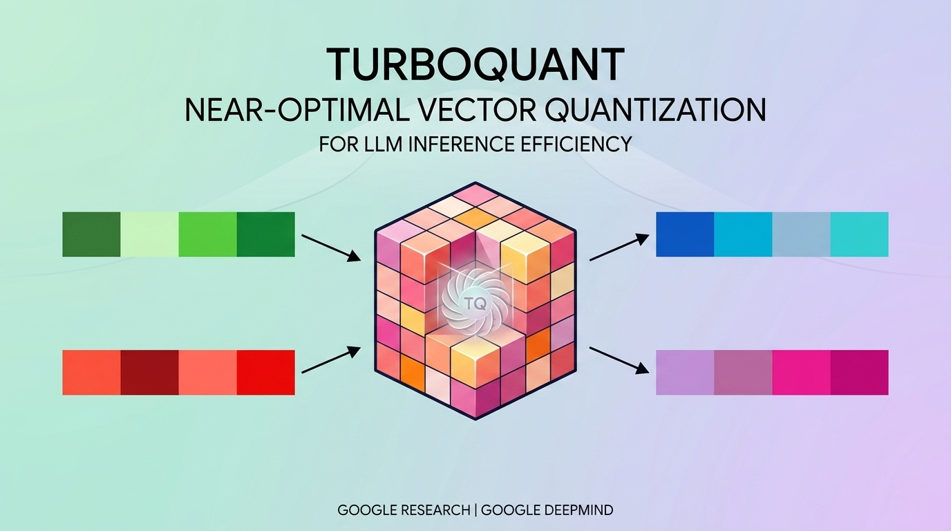
TurboQuant: Near-Optimal Vector Quantization for LLM Inference Efficiency

A deep dive into Google’s new vector quantization method that challenges the information-theoretic limits of compressing high-dimensional embeddings

Introduction

Modern large language models (LLMs) are extraordinary. They can write code, summarise documents, reason across hundreds of pages, and hold multi-turn conversations with impressive coherence. But that coherence comes at a cost: memory.

Every time a transformer model generates a new token, it needs to remember the representations of every previous token it has seen. These representations — stored in what is called the KV cache (key-value cache) — grow linearly with context length and can easily occupy gigabytes of GPU VRAM for long-context scenarios. When you are running a model with a 128k-token context window, this is no longer a footnote — it is the dominant bottleneck of inference.

The challenge, then, is clear: how do we compress the KV cache aggressively without compromising the model’s ability to answer correctly?

This is precisely the question that a team from Google Research and Google DeepMind sets out to answer in their recent paper, ”TurboQuant: Online Vector Quantization with Near-optimal Distortion Rate” (Zandieh et al., 2025). The result is a quantization algorithm that is not only theoretically grounded — it operates within a provably small constant factor of what is information-theoretically possible— but is also practically fast, GPU-friendly, and immediately applicable to real inference pipelines.

A Quick Refresher: What Is Vector Quantization?

Before diving into TurboQuant, let’s ground ourselves in the problem.

Quantization converts floating-point values to lower-precision integers. If you have a 32-bit float embedding vector of dimension 1536, naively storing it costs 1536 × 4 bytes = ~6 KB. Quantizing to 4 bits per coordinate brings that down to 768 bytes — a 8× reduction. The catch: you introduce distortion.

Vector quantization (VQ) does this holistically. Rather than quantizing each coordinate independently (scalar quantization), VQ considers the structure of the full vector and aims to minimise distortion metrics such as:

• MSE— Mean-Squared Error: how close is the reconstructed vector to the original in L2 distance?
• Inner product error — How accurately can we compute ⟨q, k⟩ from the quantised key vector? This is critical for attention mechanisms.

The gold standard for VQ is Shannon’s distortion-rate function, which tells us the minimum possible distortion achievable at a given bit budget. For decades, practical algorithms have fallen well short of this bound. TurboQuant closes much of that gap.

The Problem with Existing Approaches

Current approaches to KV cache quantisation fall into two broad camps:

1. Data-dependent (offline) methods: These, like Product Quantization (PQ), learn a codebook from training data using k-means. They can achieve good distortion but require preprocessing, are slow to index, and cannot adapt to new data on the fly — a deal-breaker for online inference where new key-value embeddings arrive at generation time.
2. Data-oblivious (online) methods: These apply fixed transformation rules without any data-specific tuning. They are fast but historically have suffered from suboptimal distortion rates.

TurboQuant targets exactly the latter category: online, data-oblivious quantisation, and proposes to make it near-optimal.

TurboQuant at a Glance

Before going into the mathematical details, it helps to build an intuition for what TurboQuant actually does — and why each step makes sense.

Imagine you need to compress a high-dimensional vector (think of it as a list of thousands of floating-point numbers) into a much more compact representation, while keeping the ability to reconstruct it with minimal error. The naive approach — just rounding each number independently — works poorly because the distribution of values in a real embedding vector is unpredictable and highly varied. Some coordinates are large, some are tiny, and the quantiser cannot know in advance what to expect.

TurboQuant solves this with a simple but powerful idea: shuffle the vector into a predictable shape before compressing it. Specifically, it applies a random rotation to the input, which spreads the information uniformly across all coordinates. After this rotation, every coordinate follows the same well-known statistical distribution — regardless of what the original vector looked like. This transforms an unpredictable compression problem into a well-understood one.

Once the distribution is known and uniform, TurboQuant applies a pre-computed optimal quantiser to each coordinate independently. Because the coordinates are nearly statistically independent after rotation (a property that holds in high dimensions), treating them separately introduces almost no extra error. The quantiser is calibrated exactly for the known distribution, squeezing out maximum efficiency at every bit-width.

There is, however, one catch: this MSE-optimal compression introduces a systematic bias when the quantised vector is later used to compute attention scores (inner products). To fix this, TurboQuant adds a second, lightweight stage: it takes the small residual error left after the first compression, and encodes it using a single additional bit per coordinate via a technique called QJL. This correction is mathematically guaranteed to be unbiased, so the final inner product estimates are accurate on average — no matter how aggressively the original vector was compressed.

The result is an algorithm with three key properties working together: a rotation that neutralises worst-case inputs, a lookup-table quantiser tuned to the resulting distribution, and a 1-bit residual correction that restores unbiasedness. The sections below unpack each of these in detail.

How TurboQuant Works

Step 1 — Randomise Away the Worst Case

The key insight behind TurboQuant is elegant: if you cannot control the distribution of your input vectors, manufacture a known distribution.

By multiplying any input vector x by a random rotation matrix Π (generated via QR decomposition of a random Gaussian matrix), the resulting rotated vector Π·x is uniformly distributed on the unit hypersphere S^(d-1), regardless of what x was. This converts a worst-case input problem into a well-characterised statistical one.

Step 2 — Exploit the Beta Distribution

Each coordinate of a uniformly distributed point on the unit hypersphere follows a known Beta distribution (which converges to a Gaussian in high dimensions). More importantly, in high dimensions, distinct coordinates become nearly independent — a fact rooted in the concentration-of-measure phenomenon.

This near-independence is the crux of the algorithm: it means we can quantise each coordinate independently using a scalar quantiser, without paying a price for ignoring inter-coordinate correlations. The problem reduces from a hard joint optimisation to d independent 1D optimisations.

Step 3 — Optimal Scalar Quantisation via Lloyd-Max

Given the known Beta distribution, the team solves the classical Lloyd-Max quantisation problem: partition the interval [-1, 1] into 2^b buckets to minimise the expected squared error. This is a 1D k-means problem, solved once offline and stored as a lookup table for any given bit-width b.

The resulting quantiser is called TurboQuant_mse. It provably achieves:

for any bit-width b and any worst-case unit-norm input vector. The information-theoretic lower bound is 1/4^b, so TurboQuant_mse is within a constant factor of √(3π)/2≈ 2.7 of the theoretical optimum — for all bit-widths and all dimensions simultaneously.

Step 4 — Fixing Inner Product Bias

There is a subtlety that the paper addresses head-on. MSE-optimal quantisers are biased when used for inner product estimation. At 1 bit, the bias is a multiplicative factor of 2/π — meaning ⟨q, k⟩ is systematically underestimated. This is problematic for attention scores, which depend on accurate inner products.

The fix is a two-stage approach that gives rise to TurboQuant_prod:

1. Apply TurboQuant_mse with bit-width b-1 to get an initial reconstruction x̃_mse and the residual r = x — x̃_mse.
2. 2. Apply a 1-bit QJL (Quantized Johnson-Lindenstrauss) transform to the residual r.

The QJL transform — introduced in an earlier paper by the same team — produces an unbiased estimator of ⟨y, r⟩ by computing sign(S·r) where S is a random Gaussian matrix. The final dequantised estimate is:

This composition is unbiased (by design of QJL) and inherits the small residual norm from the MSE stage. The inner product distortion bound becomes:

which again is within a constant of the theoretical lower bound of

What the Experiments Show

The paper validates TurboQuant on three fronts.

Distortion Validation

On the DBpedia Entities dataset (1536-dimensional OpenAI embeddings), both TurboQuant_mse and TurboQuant_prod closely match the theoretical distortion bounds across all bit-widths from 1 to 5. TurboQuant_prod correctly exhibits zero bias in inner product estimation at all bit-widths, while TurboQuant_mse shows decreasing bias as bit-width increases.

Figure 3 from Zandieh et al. (2025): Observed inner-product error (left) and MSE (right) plotted alongside theoretical upper and lower bounds across bit-widths. Both variants of TurboQuant closely track the bounds. ((https://arxiv.org/abs/2504.19874), CC BY 4.0)

KV Cache: Needle-in-a-Haystack

sing Llama-3.1–8B-Instruct, the model’s long-context recall is tested at context lengths from 4k to 104k tokens with a 4× memory compression ratio. TurboQuant achieves a perfect score of 0.997 — identical to the full-precision baseline — while methods like SnapKV (0.858) and KIVI (0.981) fall noticeably behind.

Figure 4 from Zandieh et al. (2025): Needle-in-a-Haystack recall heatmaps for Llama-3.1–8B-Instruct across context lengths (4k–104k tokens) at 4× compression. Darker regions indicate retrieval failures. TurboQuant matches full-precision across all context lengths. ((https://arxiv.org/abs/2504.19874), CC BY 4.0)

KV Cache: LongBench End-to-End Generation

On LongBench-E with Llama-3.1–8B-Instruct, TurboQuant at 3.5 bits matches the full-cache score of 50.06 exactly, while the competing PolarQuant at 3.9 bits reaches only 49.78. At an aggressive 2.5 bits (with outlier-channel handling), TurboQuant achieves 49.44 — a marginal drop, representing a >6× compression ratio.

Nearest Neighbour Search

TurboQuant consistently outperforms both PQ and RabitQ in recall@1@k across GloVe (d=200), DBpedia-1536, and DBpedia-3072 datasets, at both 2-bit and 4-bit precision. The gap is particularly pronounced at lower top-k values, which is where real-world ANN systems operate.

The speed comparison is striking: at d=3072 with 4-bit quantisation, TurboQuant takes 0.002 seconds to index 100k vectors, versus 494 seconds for PQ and 3957 seconds for RabitQ. This essentially eliminates the indexing overhead entirely.

Figure 5 from Zandieh et al. (2025): Recall@1@k comparison of TurboQuant, Product Quantization, and RabitQ across three datasets at 2-bit and 4-bit precision. TurboQuant consistently dominates, especially at low top-k values. ((https://arxiv.org/abs/2504.19874), CC BY 4.0)

Strengths

1. Near-optimal, formally proven distortion. This is rare. The paper provides both upper bounds (via TurboQuant’s construction) and lower bounds (via Shannon + Yao’s minimax), and the gap between them is a small constant. This gives practitioners a reliable guarantee: you know exactly how much distortion you are accepting.
2. Truly online and data-oblivious. No training set, no codebook fitting, no warm-up phase. The random rotation matrix is generated once and reused. This makes TurboQuant the first method suitable for streaming KV cache quantisation during live inference.
3. Accelerator-friendly. The algorithm is fully vectorisable: matrix multiplications, sign operations, and nearest-centroid lookups all parallelise naturally on GPUs and TPUs. This is in sharp contrast to grid-based methods like RabitQ, which rely on binary search and lack GPU vectorisation.
4. Unbiased inner product estimation. The two-stage TurboQuant_prod guarantees that attention score estimates are not systematically biased, which is critical for maintaining model accuracy — especially at aggressive compression rates.
5. Negligible indexing time. In vector database scenarios, TurboQuant’s encoding step is so fast it essentially costs nothing, removing a major operational pain point of existing PQ-based systems.

Weaknesses and Limitations

1. A constant-factor gap remains. While the ≈ 2.7 factor over the information-theoretic optimum is the best known for any online algorithm, it is still a gap. For extremely memory-constrained deployments (e.g., 1-bit quantisation on very large models), this overhead may not be acceptable.
2. Additional storage overhead for inner product quantisation. TurboQuant_prod stores the MSE-quantised index, the QJL sign vector, and the residual norm γ. Compared to pure MSE quantisation, this is a richer representation and may complicate memory layout in tight inference kernels.
3. The random matrix S is large. The QJL transform requires a d×d Gaussian matrix, which for d=4096 (common in modern LLMs) is 64M float32 values — roughly 256 MB just for the projection. While this is a one-time setup cost, it must reside in GPU memory throughout inference.
4. Outlier treatment adds complexity. The non-integer bit-widths reported in the LongBench experiments (2.5-bit, 3.5-bit) require splitting channels into outlier and non-outlier sets and applying TurboQuant independently to each. This is not inherently complex, but it introduces an engineering layer that the core algorithm does not address.
5. Limited head-to-head comparison on ANN. The nearest neighbour experiments compare against PQ and RabitQ but not against more recent learned, data-dependent methods that have been specifically tuned for high-dimensional inner product search. The advantage of TurboQuant on datasets with very specific structure (e.g., GloVe d=200) is also less pronounced.

Why This Matters for AI Infrastructure

The trend in LLM development is unambiguous: models are getting larger, context windows are getting longer, and inference costs are the dominant operational expense for most enterprise deployments. Techniques that can reduce KV cache memory by 4–6× without measurable quality loss have immediate, concrete dollar value.

What makes TurboQuant stand out is not just the performance numbers but the theoretical foundation. Most quantisation papers present empirical improvements; TurboQuant provides a formal proof that its approach is near-optimal, which means practitioners can reason about the trade-offs with confidence rather than treating the method as a black box.

For teams building RAG pipelines, vector databases, or LLM inference infrastructure, TurboQuant represents a strong candidate to replace or augment existing quantisation layers — especially where online encoding speed is a priority.

Conclusions

TurboQuant is a clean, theoretically grounded solution to a very practical problem. By combining random rotation, Beta-distribution-optimal scalar quantisation, and the QJL residual correction, it achieves near-optimal distortion for both MSE and inner product metrics, with essentially zero indexing time and full GPU vectorisation.

Its main trade-offs — a constant factor above the information-theoretic optimum, extra storage for the QJL component, and a large random projection matrix — are well understood and manageable in most deployment scenarios.

As LLM context windows push towards millions of tokens, the pressure on KV cache efficiency will only intensify. Approaches with the formal guarantees and operational simplicity of TurboQuant are not just academically interesting: they are likely to become infrastructure primitives.

References: Zandieh, A., Daliri, M., Hadian, M., & Mirrokni, V. (2025). TurboQuant: Online Vector Quantization with Near-optimal Distortion Rate. arXiv:2504.19874.