Q Learning vs SARSA

Q-learning

In 1989, a revolutionary reinforcement learning (RL) algorithm called Q-learning was introduced, significantly accelerating RL progress. Q-learning was special because it enabled agents to not only evaluate immediate actions but also actively consider future states, making it easier for mathematicians to prove convergence towards optimal policies. Let’s unpack Q-learning step-by-step, clarifying its workings, benefits, and practical implementation.

The fundamental component of Q-learning is the Action-Value function Q(s,a):

• It estimates the expected return (reward) from choosing action a in state s.
• Over time, Q-learning updates these estimates to become increasingly accurate, converging toward optimal values.

Mathematically, the core of Q-learning is represented as follows:

Q-learning online update rule to estimate the expected return

Breaking down the equation intuitively:

• Q(s,a): Current estimate of expected return for state-action pair (s,a).
• α: Learning rate, controlling the rate of value updates.
• r: Immediate reward received after action a.
• γ: Discount factor, weighting future rewards.
• max⁡a′Q(s′,a′): Optimal estimated future return (looking ahead one step).
• s’: Next observed state after action a.

The term in brackets, r+γmax⁡a′Q(s′,a′)−Q(s,a), is called the TD error. It measures how “wrong” the current prediction is compared to actual experience. Each update nudges the estimate closer to reality.

Input: A policy (e.g., ε-greedy) which uses action value function
Initialize Q-table Q(s, a) arbitrarily (e.g., all zeros)
For each episode:
    Reset environment to initial state s

    While s is not terminal:
        Choose action a from s using policy, breaking ties randomly
        Execute action a, observe reward r and next state s'

        # Q-value update rule
        Q(s, a) ← Q(s, a) + α [r + γ max_a' Q(s', a') - Q(s, a)]

        Move to next state s'

End

With sufficient episodes, the Q-values approach optimal action-value estimates, guiding increasingly effective decisions.

Tabular Q-Learning: Strengths and Limitations

The original Q-learning implementation is tabular, meaning it explicitly stores action-value estimates in a table indexed by state-action pairs. Advantages: Simple, intuitive, mathematically provable convergence in discrete settings. Limitations: Impractical for continuous states or actions because the table size grows infinitely. Modern approaches (like Deep Q-Networks) use neural networks instead of tables to handle continuous problems.

What Makes Q-learning Special?

Q-learning is a form of Temporal-Difference (TD) learning, therefore it also combines two critical concepts, Sampling and Bootstrapping. What distinguishes Q-learning from previous methods is its ability to:

• Look ahead (rollout): The algorithm scans all potential future actions (a’) from the next state (s’). It selects the best future action, thus guiding the agent towards trajectories that promise higher rewards. Instead of choosing actions based solely on immediate rewards, Q-learning guides decisions towards optimal long-term strategies. This capability allows Q-learning agents to effectively “predict the future,” crafting plans that maximize long-term cumulative rewards.
• Be off-policy: Q-learning is a classic example of an off-policy algorithm. It updates values based on the optimal action possible, regardless of the current action selection policy. This flexibility allows agents to learn effectively, even while employing exploratory policies (like ε-greedy) that don’t always take the optimal action. This subtle yet crucial capability enables more effective and flexible learning, increasingly valuable in complex, uncertain environments.

Off-policy: The algorithm learns value estimates independently of the current policy.

Practical Applications and Extensions

Q-learning serves as a foundational method, underpinning modern advancements like:

• Deep Q-Learning (DQN): Combines Q-learning with neural networks, handling high-dimensional states (e.g., image pixels in Atari games).
• Policy improvement: Enables agents to iteratively refine policies toward global optimality, achieving impressive results in robotics, gaming, finance, and automation.

SARSA

Shortly after Q-learning revolutionized reinforcement learning (RL), another powerful algorithm called SARSA was developed. SARSA addressed some subtleties of Q-learning, making it more general and adaptable. But what exactly is SARSA, how does it differ from Q-learning, and why should we care?

SARSA is a Temporal-Difference (TD) learning algorithm, named after the sequence it uses to perform updates:

S (State) → A (Action) → R (Reward) → S’ (Next State) → A’ (Next Action)

In other words, SARSA updates action-values based on:

The current State and Action, the observed immediate Reward, and the next State and Action.

Unlike Q-learning (an off-policy algorithm), SARSA is explicitly on-policy:

• On-policy means the agent learns action-value estimates directly from the actions it actually takes.
• The policy being evaluated (improved) and the policy used to generate the data are the same.
• SARSA explicitly uses the next action (chosen by the current policy) in its updates.

This subtle change affects how SARSA behaves practically, particularly in scenarios with risk, exploration, and uncertainty.

Input: A policy (e.g., ε-greedy) which uses action value function
Initialize Q-table Q(s, a) arbitrarily (e.g., all zeros)
For each episode:
    Reset environment to initial state s

    While s is not terminal:
        Choose action a from s using policy, breaking ties randomly
        Execute action a, observe reward r and next state s'
        Choose action a' from s' using policy, breaking ties randomly

        # Q-value update rule
        Q(s, a) ← Q(s, a) + α [r + Q(s', a') - Q(s, a)]

        Move to next state s'
        Move to next action a'

End

SARSA vs. Q-Learning: What’s the Difference?

The core difference lies in how these algorithms handle future actions:

Q-Learning (Off-policy):

• Considers the best possible action from the next state, regardless of the current policy.
• Uses argmax to select the action with the highest future reward potential:

Q-learning online update rule to estimate the expected return

SARSA (On-policy):

• Uses the actual next action (chosen by the current policy), without argmax:

SARSA online estimate of the action-value function

Key Differences Between Q-learning and SARSA

Q-Learning (Off-policy)

Action Evaluation: Evaluates returns by assuming that the agent always selects the optimal action in future steps. Idealistically expects no accidental or random exploratory actions.

Learning Data: Off-policy, allowing the agent to learn from data collected under any policy. Enables greater flexibility in data reuse and efficiency.

Behavioral Result: Tends to learn riskier, aggressive strategies that aim for ideal optimal paths. Potentially unstable when exploring, as it doesn’t account for occasional exploration-related mistakes.

SARSA (On-policy)

Action Evaluation: Evaluates expected returns based on the actions the agent actually takes, including exploratory moves. Explicitly considers randomness and risks introduced by exploration policies.

Learning Data: On-policy, meaning it learns from data gathered from the current exploration policy. Limits data reuse but typically provides more stable policy improvement.

Behavioral Result: Tends to learn safer, cautious policies, explicitly accounting for occasional exploratory slips or mistakes. More stable during exploration, offering greater reliability in risk-sensitive environments.

Gridworld Cliff Example: Q-learning vs. SARSA

The Gridworld environment — particularly the cliff-walking variant — is a classic example in RL literature illustrating practical differences clearly:

Scenario Setup: A two-dimensional grid where the agent must navigate from a start state to a goal state. It has a hazardous “cliff” area: stepping off results in a large negative reward.

Reward Structure:

• Regular step: Reward = −1
• Falling off cliff: Reward = −100 (ends episode)
• Goal state reached: Reward = 0 (ends episode)

A depiction of the grid environment with a cliff along one side

Results:

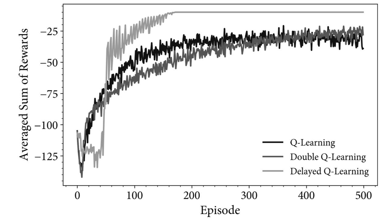
A comparison of Q-learning against SARSA for a simple grid problem

Q-Learning Behavior (Off-policy)

• Predicts future rewards assuming the agent will always pick the optimal action.
• Prefers the shortest, ideal path along the cliff edge.
• Ignores risk of random exploratory actions causing accidental falls off the cliff.
• Results in occasional catastrophic failures, producing unstable rewards due to significant penalties from accidental falls.

SARSA Behavior (On-policy)

• Predicts future rewards based on actual actions taken, including random exploratory moves.
• Prefers a slightly longer, safer path away from the cliff.
• Explicitly considers risk, reducing likelihood of random exploratory actions causing dangerous falls.
• Provides more stable, consistent performance.

The policies derived by Q-learning and SARSA agents. Q-learning tends to prefer the optimal route. SARSA prefers the safe route.

These differences have significant implications in practical, real-world applications:

Application: Self-Driving Cars

Q-Learning (Off-policy) — Aggressively chooses the shortest route, disregarding occasional exploratory risk (higher risk of accidents). SARSA (On-policy) — Prefers safer routes, actively avoiding risks of accidents during exploration.

Application: Robotics

Q-Learning (Off-policy) — Learns aggressive, optimal strategies without accounting for accidental errors (ideal but risky). SARSA (On-policy) — Learns cautious, stable strategies accounting explicitly for occasional exploratory mistakes (safe, stable).

Conclusion

Two popular TD algorithms — Q-learning and SARSA — highlight critical differences in learning approaches: Q-learning, an off-policy method, optimistically estimates future rewards by assuming optimal action selection, leading to aggressive but riskier policies; whereas SARSA, an on-policy method, realistically evaluates future rewards based on the agent’s actual behavior, leading to safer, more stable policies. Choosing between them depends on practical requirements: prioritize Q-learning for flexibility, efficiency, and idealized optimality, or SARSA for stable, cautious policies in scenarios sensitive to exploration risks.