Part 1: Geospatial AI is changing how we see the world.

What are the representations that power these geospatial models? What you can do with them? In this series we will break down the latest work at NatureAlpha on forecasting nature-related changes (funded by AWS facilitated by ThriveGEO).

AlphaEarth Foundations (Google, 2025)

An enormous amount of data has been collected about places on Earth. For any patch of ground you can pull optical imagery across a dozen spectral bands, radar, lidar, and repeat passes through the year, from several satellites. Stack it all up and a single location becomes dozens of layers, each with its own resolution, units, and quirks.

Most of that is redundant. A forest looks like a forest across nearly all of those channels, year after year. So the obvious question: can we compress it? Can we boil down everything we know about a place into something small enough to actually work with, without throwing away what matters?

That’s what a geospatial foundation model does. Geospatial foundation models take a full year of Earth observation data and squeezes it, for every 10-metre or 30-metre spatial resolution. Google’s AlphaEarth Foundations (AEF) summarises all the data in a vector of 64 dimensions (this number varies depending on the foundation model that you use).

What the embedding dimensions represent

Its key to understand how models represent the data. The natural assumption is that those 64 numbers (in the case of Google’s model) are measurements: that one of them is “greenness,” another “moisture,” another “built-up area.” They aren’t. No single number means anything on its own, and you can’t read a vector and say what’s on the ground.

What the numbers encode, taken together, is similarity. The model was trained so that two pixels that look alike (same land cover, same condition, same seasonal rhythm) get vectors that sit close together, and two pixels that differ end up far apart. It just learned to place look-alikes near each other and push everything else away.

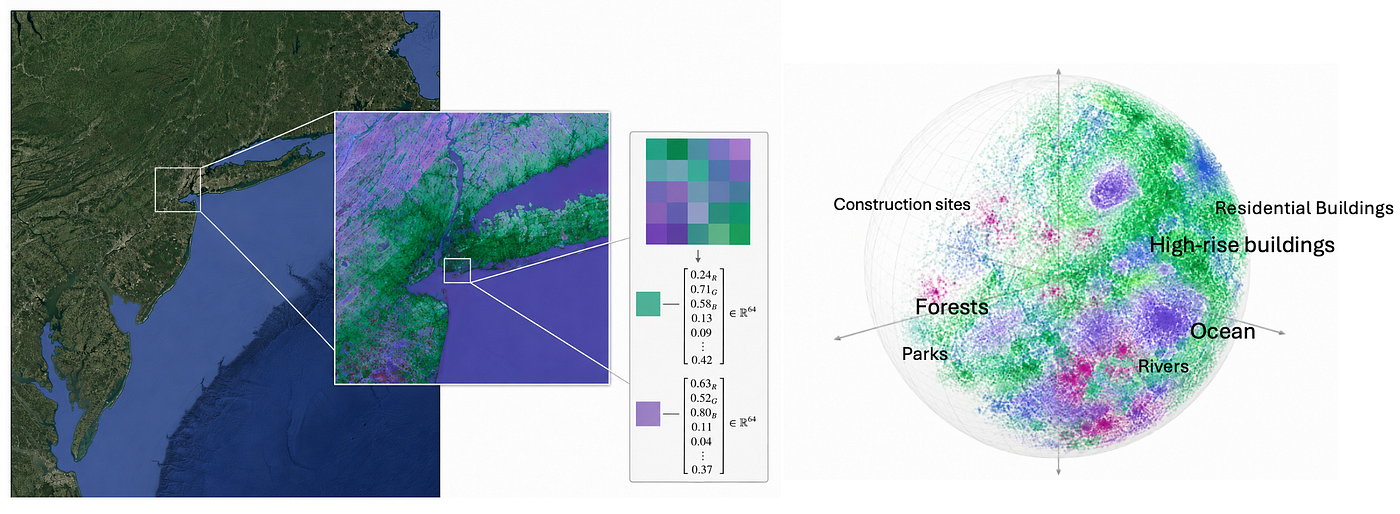
Figure 1: Schematic of Geospatial Foundation Models (AEF; Alpha Earth Foundations, Google). Left: AEF represent the earth at 10m resolution. In the middle image of the schematic you see houses have similar colours (green), water has similar colours (dark purple), woodlands in also have similar colours (light purple); the colours represent the similarity of information that those 10m pixels have with other pixels. Right: If we look how the AEF represents the data, the closest similarity would be the image on the right (its hard to show a 64-dimensional sphere so this has to do. We see all the pieces of land that show similar types of data grouped together.

The easiest way to picture this is the result, not the mechanism. Think of every pixel on Earth as a single dot, and arrange all those dots in a space where distance means dissimilarity. You don’t get a scatter of noise. You get a structured map (see figure above, where I try to show a 64 dimensional sphere). All forest-like places occupy related neighbourhoods in the embedding space, while croplands, wetlands, urban areas, and other land-cover types tend to separate to different parts of the representation. Similar land covers sit near each other even when they’re on opposite sides of the planet. A pine forest in Canada lands near a pine forest in Sweden, because they look and behave alike, not because they’re geographically close.

This is the idea the rest of the series rests on, so it’s worth emphasising. The embedding is a similarity space. It isn’t a picture of a place. It’s a coordinate that says where this place sits among all other places on Earth. The meaning lives in the layout: which neighbourhood a point falls into, and which other points surround it.

What do you mean, similarity space?

A few facts about how that space is built will be very important later on:

The data points from the AlphaEarth model are all the same length (they’re scaled to sit exactly one unit from the centre), so every pixel lands not just anywhere in the space but on the surface. That sounds like a technicality, but it changes how you measure closeness: you compare two pixels by the angle between their directions from the centre, not by straight-line distance. Two places are alike if they point the same way.

Figure 2: Similarity between points is usually measured in angle, not direct (euclidean) distance between the dots directly.

This is useful for various reasons, a few straightforward implementations are:

• Similarity Search: finding 10m pixels that look very similar to the selected pixel (left, figure 3). Its a very effective way to for example find all the grain silo’s in the united states, mining sites, cattle farms, solar panels.
• Change detection: detecting how much the angle has shifted over time provides a useful indication of change in land cover (right, figure 3). See this google blog for an example.

Figure 3: Putting Embeddings to Use. Left: Vector similarity search. Right: Change detection for two locations, the bottom pair changes a bit more (purple) then the top pair (blue).

The next part will look more closely at changes over time and how we can interpret those better in the context of geospatial AI data representations!