Photo by Aaron Burden on Unsplash

Where patterns repeat, and the future quietly echoes the past

It’s been a long time I did not touch a times series analysis, I know that maybe one year ago I wanted to build a series around it covering and if you are a bit cusious like me a deep dive in the backbond behind the models

I had a job to do for a friend related to that and while doing it I rememberded my intention to cover it ! in that article I will cover Naive Seasonal models and everything you need to know about it !

As always, if you find my articles interesting, don’t forget to clap and follow 👍🏼 These articles take time and effort to create!

The intuition behind the Naive Seasonal Model

Before diving into any complex models like ARIMA, Prophet, and so on, it’s important to establish a baseline, and the Seasonal Naive model is one of the most important benchmark models for data that exhibits cyclical patterns

The intuition behind the model can be summarized in one sentence: “History repeats itself exactly one season later”

To understand this well, I will go classical to make it quick, let’s say you run an ice cream shop. To predict your sales for July of this year, you wouldn’t look at your sales from June (which is just the start of summer), nor your sales from December (when it’s cold)

The best simple estimate you can make is to look at your sales from July of last year and assume you will make the exact same amount

This is an extremely effective approach for data heavily dominated by seasonality (weather, holiday sales, rush hour traffic…)

You can check my previous article for an introduction to time series analysis

[embed]Introduction to Time Series Analysis Introduction to Time Series Analysis This is the first article in a series on forecasting. I'm sure you've already…ai.plainenglish.io

What’s the math behind the model ?

If you are always curious about how things work, I will explain everything you need to know. As you may understand from the intuition, the Seasonal Naive model states that the forecast for time T+h is equal to the last observed value at the same season

• T: The current time (the end of your training data)
• h: The forecast horizon (how many time steps ahead you are predicting)
• m: The seasonal period (ex : m=12 for months, m=4 for quarters)
• Yt : The actual observed value at time t
• y-hatT+h|T: The predicted value for time T+h given the data up to T

The equation is written as follows :

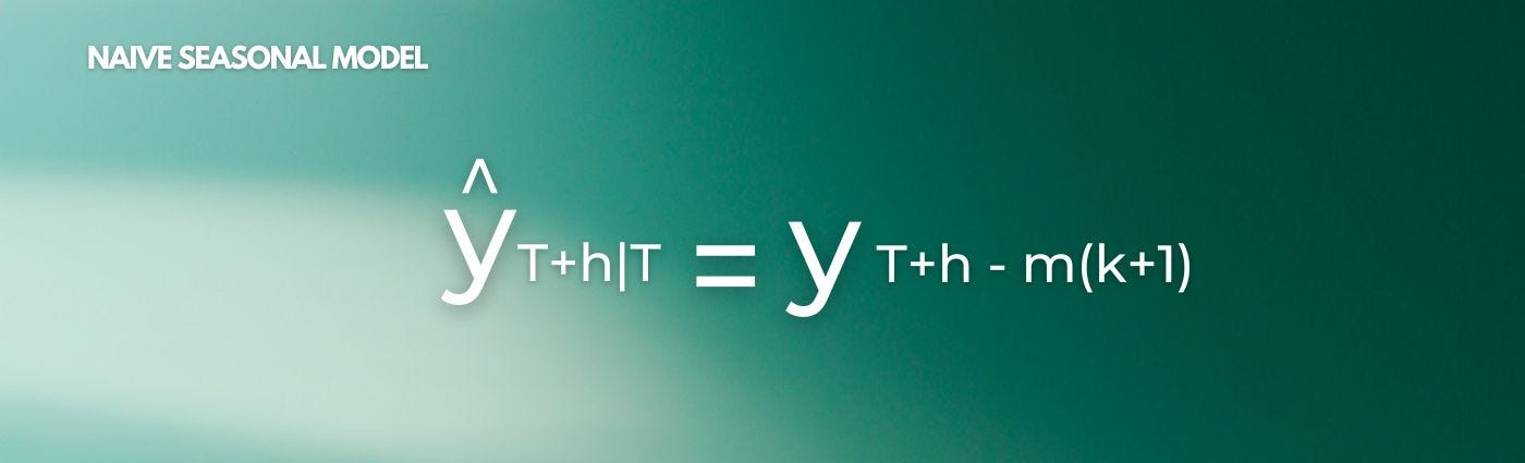
Naive Seasonal Model. Image Source : Dr. Walid Soula

How about k Right ?It’s the integer part of the ratio that allows us to go back to the correct previous seasonal cycle

k for Naive Seasonal Model. Image Source : Dr. Walid Soula

Note: some references write this as yt+h−km with the same k; both forms are equivalent

To get an idea of what I am talking about, let’s take an example:

• Let’s assume you are tracking quarterly sales (m=4 ; Since there are 4 quarters in a year: Q1, Q2, Q3, Q4)
• T is your present moment. Let’s say T is the end of Q4 2023

How do we predict sales for future quarters, and how does the formula ensure we always pick the correct historical quarter? (seasonality cases, of course)

Let’s predict Q2 2024. We first need k. It is 2 steps in the future, so h=2

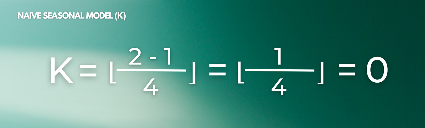
Note: Keep in mind that you have a floor function, which always rounds down to the nearest whole integer. That’s why you have k=0

Since k=0, it means we don’t need to jump back any extra years; we just look at the immediate past year. Then let’s plug k into the main formula

So, if T is Q4 2023, then T−2 is exactly Q2 2023. The math correctly selects the same quarter from the previous year for the target Q2 2024

Parameters of the model

As you may have read so far, the major advantage of this model is its simplicity: no gradient descent or weight optimization. It has only one explicit parameter that the user must provide, and that is the seasonal period (m)

That seasonal period is defined by the length of the cycle. If you omit this parameter or set it incorrectly, you will get poor results

• Hourly data (daily cycle): m = 24
• Daily data (weekly cycle): m = 7
• Monthly data (annual cycle): m = 12
• Minutely for Hourly 60
• Minutely for Daily 1440
• …

Note : You can find “m” in some texte book as “sp”

You will certainly not do the computation by hand, and you will probably use Python or maybe an LLM to handle it for you. Let’s have a quick example in Python

1 — The Imports and Generating the Synthetic Data

Before starting, we bring in the standard data science toolkit and generate synthetic data (3 years of data)

Note: The series will have seasonality (sine wave), a slight trend, and some noise

import pandas as pd
import numpy as np
import matplotlib.pyplot as plt

np.random.seed(42)
dates = pd.date_range(start='2020-01-01', periods=36, freq='ME')

# Create a series with seasonality (sine wave), a slight trend, and some noise
seasonality = np.sin(np.arange(36) * (2 * np.pi / 12)) * 50
trend = np.arange(36) * 2
noise = np.random.normal(0, 5, 36)
sales = 100 + seasonality + trend + noise

df = pd.DataFrame({'Date': dates, 'Sales': sales}).set_index('Date')

2 — The Train / Test Split

For training, I will take everything from the beginning up to the last 12 months, and for testing, I will use the last 12 months

train = df.iloc[:-12]
test = df.iloc[-12:]

3 — Applying the Seasonal Naive Model

We don’t need machine learning libraries here. Since we want to predict the next 12 months and our seasonal cycle is exactly 12 months, you can also add a visualization

m = 12
forecast = train.iloc[-m:].copy()
forecast.index = test.index # Align dates with the test set
forecast.columns = ['Naive_Forecast']

# Visualize the results
plt.figure(figsize=(12, 6))
plt.plot(train.index, train['Sales'], label='Training Data', color='blue')
plt.plot(test.index, test['Sales'], label='Ground Truth (Test)', color='green')
plt.plot(forecast.index, forecast['Naive_Forecast'], label='Seasonal Naive Forecast', 
         color='red', linestyle='--')

plt.title('Sales Forecasting with the Seasonal Naive Model')
plt.xlabel('Date')
plt.ylabel('Sales')
plt.legend()
plt.grid(True, alpha=0.3)
plt.show()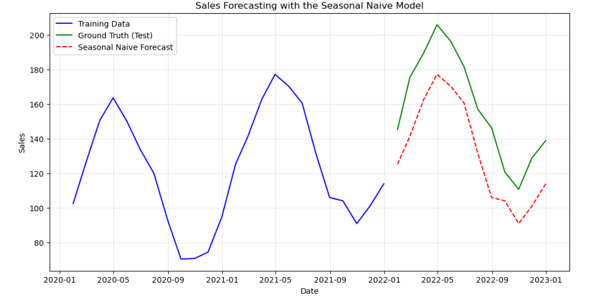

Sales Forecasting with the Seasonal Naive Model. Image Source : Dr. Walid Soula

• Blue Line (Train): The historical data the model gets to “see”.
• Green Line (Test): The actual reality of what happened in the 3rd year.
• Red Dashed Line (Forecast): Our Seasonal Naive prediction

4 — Evaluating the Error

I will use MAE. By that, I mean we will subtract our forecasted values from the actual test values, take the absolute value (so negative and positive errors don’t cancel each other out), and calculate the average

mae = np.mean(np.abs(test['Sales'] - forecast['Naive_Forecast']))
print(f"The Mean Absolute Error (MAE) of the naive model is: {mae:.2f}")
# The Mean Absolute Error (MAE) of the naive model is: 25.99

MAE. Image Source : analyticsvidhya

The question you may have is: how do I interpret the result? Is it good or bad? The short answer is that there is no universal “good” number. An MAE of 26 is fantastic if you are selling 10,000 cars a month, but it is catastrophic if you only sell 30! However, you can use Mean Absolute Percentage Error (MAPE), which will help you understand the result better relative to your specific data

mape = np.mean(np.abs((test['Sales'] - forecast['Naive_Forecast']) / test['Sales'])) * 100
print(f"The Mean Absolute Percentage Error (MAPE) is: {mape:.2f}%")
# The Mean Absolute Percentage Error (MAPE) is: 16.77%

The Universal Rule of Thumb for MAPE:

• Less than 10%: Highly Accurate. This is an excellent model (It can be safely used for strict financial planning, budget allocation, and sensitive supply chain management)
• 10% to 20%: Good / Acceptable. This is the sweet spot for most standard business forecasts (Our Seasonal Naive model scored 16.77%, putting it solidly in this category! It is highly useful for general strategic planning)
• 20% to 50%: Fair / Needs Improvement. The model is capturing some patterns, but it is missing the mark too often (You should not rely on this for critical business decisions without human oversight)
• Greater than 50%: Unacceptable / Poor. A model in this range is practically guessing (You are better off flipping a coin or investigating your data for severe errors)

Missing trend ?

A 16.77% error is good, but if we look closely at our data, we can understand exactly why the model was off by an average of 25.99 sales.

Remember when I generated our synthetic data in Python? I intentionally added a trend that grows the business by exactly 2 sales every month:

trend = np.arange(36) * 2

Because the standard Seasonal Naive model simply repeats values from exactly 12 months ago, it completely ignores the fact that the business is growing; it misses the accumulated growth over time.

Seasonal Naive models are excellent at capturing repeating patterns, but they fail when the data has a clear long-term trend.

How do we handle the trend? The Drift Method

To account for this limitation, we can use a simple baseline approach called the Drift method.

WRC Red Bull.Image Source : redbull

That’s not exactly Drift; if your data has an obvious overall direction (growing or shrinking), you should use the Seasonal Naive with Drift model.

Instead of just saying, “History repeats itself exactly,” this model says: “History repeats itself, but we also recognize that the business is growing by an average amount with every single step.”

Instead of assuming only repetition, Drift assumes a constant average change over time. This average change per time step is computed as: YT-Y1/T-1 . Let’s define this value as x

This represents the global trend of the series. We estimate the average change per time step x and project it forward over h steps as h × x .So, the full Drift model formula becomes: YT + h×x

Note :

• YT​: The last observed value in your time series (at time T)
• Y1 : The first observed value in your dataset
• T : The time index of the last observation (If you have 36 data points, then T=36)
• h : The forecast horizon
• x : The average change per time step (global trend)

I think that’s enough for this episode of the series. The goal here was not just to throw Python code and math formulas at you, but to help you understand the core intuition behind forecasting and why establishing a solid baseline is absolutely critical (sometimes, the simplest model can be incredibly effective).

If there’s a specific subject you’d like us to cover, please don’t hesitate to let me know! Your input will help shape the direction of my content and ensure it remains relevant and engaging 😀

Resources

[embed]List: Data Science Digest | Curated by Dr. Walid Soula | Medium Data Science Digest · Explore my curated playlist of essential Data science articles, covering topics from machine…medium.com

[embed]Dr. Walid Soula - Medium Read writing from Dr. Walid Soula on Medium. AI & Marketing Expert in Healthcare industriesmedium.com

Please consider the following and subscribe to the newsletter for more articles about business, data science, machine learning, and extended reality, it’s FREE! You can find my lists in the following links :

• Data Science Digest : https://medium.com/@soulawalid/list/statistics-data-science-65305693779d
• Generative AI : https://medium.com/@soulawalid/list/generative-ai-ee31117869a9
• Programming with Python : https://medium.com/@soulawalid/list/programming-c0a3ef000f5f
• Linguistic AI Lab : https://medium.com/@soulawalid/list/linguistic-ai-lab-9eb7d30369c1
• Strategic Business Intelligence : https://medium.com/@soulawalid/list/strategic-business-intelligence-1528f08575a7
• AI for Health Professionals : https://medium.com/@soulawalid/list/ai-for-health-professionals-f8b87eeab19f
• The Neuroscience of Consumer Behavior : https://medium.com/@soulawalid/list/the-neuroscience-of-consumer-behavior-8f94149e3c73
• Beyond Reality : https://medium.com/@soulawalid/list/beyond-reality-bf03607b0b80
• Quantum Leap : https://medium.com/@soulawalid/list/quantum-leap-be0b06f7a986

If you have any questions, you can ask me on LinkedIn, here is my profile: https://www.linkedin.com/in/oualid-soula/ Let’s connect!