Stabilizing AI Training Using a New Manifold Interpolation Method

Improving Optimization via Smooth Transitions on Learning Manifolds

AI Training is Extremely Chaotic.

Most AI research focuses primarily on final performance, measured by metrics such as accuracy, loss, and reward.

However, in practice, unstable gradients, jerky parameter updates, oscillation, and overshoot significantly impact training stability, time to convergence, reliability in deployment, and the generalization of models.

Large models, especially those with complex structures, suffer from violent learning trajectories, rapid swings, unstable direction changes, and chaotic motion across parameter space.

The core question driving this project can be reformulated into the following research hypothesis:

“Smoothing the optimization path of AI learning on manifolds enhances the predictability of learning, improves stability and efficiency in training, contributing to a superior model generalization in practical applications.”

Manifold-Constrained Learning as a Stability Tool

AI parameters often naturally lie on curved spaces (manifolds) such as:

• rotation groups (SO(3))
• directional vectors (S²)
• covariance matrices (SPD)
• low-rank embeddings for LLM fine-tuning

Constraining updates to a manifold is like guiding a child, not restricting them, but shaping how they move through learning.

This work focuses on enhancing how AI navigates, not just where it ultimately ends up.

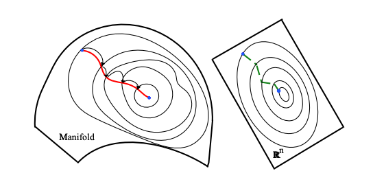
A curve flowing smoothly along a surface vs. a jagged line in open space.

What Current Manifold-Interpolation Methods Taught Me (SLERP, SQUAD, SENO)

Instead of starting with my idea, I replicated existing methods and treated them as optimization behaviors, not robotics tools.

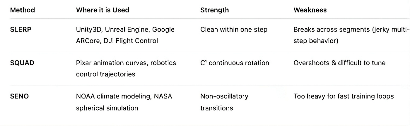
I studied 3 well-established smoothing frameworks, SLERP, SQUAD, and SENO:

SLERP Has Local Smoothness But Fails Over Several Points

SLERP, Spherical Linear Interpolation, is widely used for quaternions in AR/VR cameras and drones (DJI). It transitions smoothly between two orientations, which is good per step; however, multi-segment sequences produce slope discontinuities, as shown in the figure below.

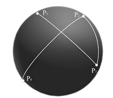
This is analogous to gradient descent, which performs well for a single update, but then becomes unstable.

SQUAD Smooths Transitions, But is Computationally Intensive

Used in Pixar animation pipelines and Unreal motion blending, SQUAD reduces the harsh corners that SLERP suffers from. However, it relies on repeated applications of Spherical Linear Interpolation (SLERP) segments smoothly connected by fillet tracts (polynomial motion laws). While SLERP itself is effective, the chained, iterative nature required for smooth higher-order curves adds significant overhead.

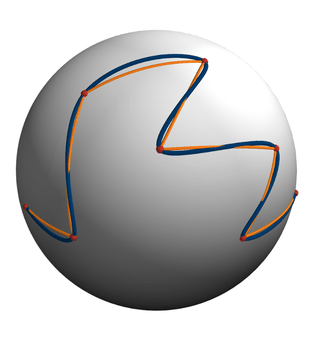
Example of the SLERP (orange) and the SQUAD (blue) interpolations between eight unit quaternions on the sphere. We can see that in contrast to the SLERP curve, the SQUAD curve overshoots between the control points (red).

In optimization terms: Its like meticulously linking many small, precise straight lines to construct a car slightly swinging wide on a turn, rather than just drawing a tight point-specific curve.

SENO Avoids Oscillation, But Isn’t Usable for Real Training

SENO is mathematically beautiful and is used by NOAA and NASA for modeling flow on spherical grids. But it requires expensive computation and doesn’t generalize to rotation groups or higher-dimensional manifolds, meaning it can only be applied to spheres.

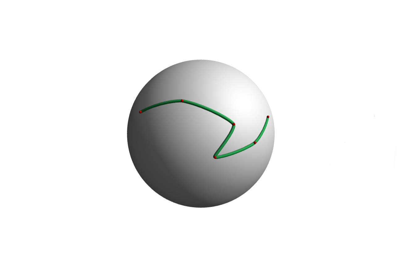
It’s stable, but not deployable in fast SGD/Adam loops.

The Gap Becomes Obvious When You See Them Together:

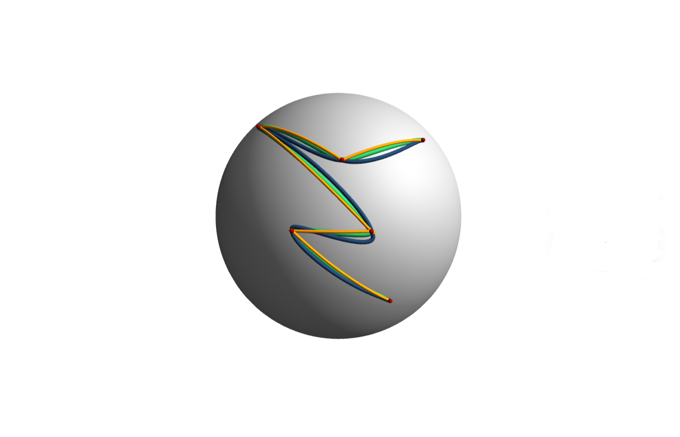
SLERP (orange) has sharp kinks, SQUAD (blue) overshoots, and SENO (green) is computationally intensive

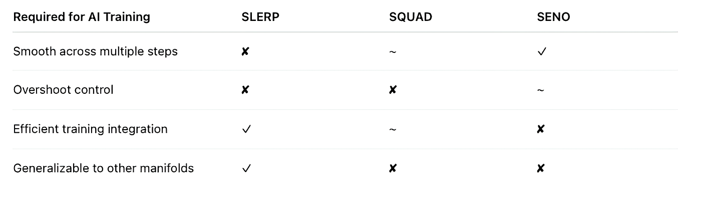
All three methods excel in one dimension and fail in another.

This brings us to Part B, which is my contribution.

My Approach: Smooth the Transitions, Not the Positions

Every existing method focuses on smoothing position interpolation. Instead, I smooth the change of direction, the kinks themselves, using a logistic smoothstep function.

A Three-Step Framework: Map to Tangent, Blend, Map Back to Manifold

1. Convert the manifold update into the tangent space
2. Apply logistic blending to derivative transitions
3. Map back to manifold via Exp()

This produces global continuity rather than local-only smoothness, single-parameter overshoot control, and compatibility with SGD/Adam training loops, as well as generalization to S², SO(3), SPD, and beyond.

Deep Dive

The core innovation lies not in smoothing positions directly but in controlling how linear connections transition across segments, maintaining accuracy, locality, and improving differentiability, all while providing direct ringing control. This approach leverages the fundamental structure of Riemannian geometry and retains the computational efficiency necessary for modern optimization.

Step 1: Convert Manifold Updates to Tangent Space

The first step establishes a local Euclidean workspace where standard calculus applies, regardless of the manifold’s global curvature.

Computing the Fréchet Mean

We begin by identifying a reference point μ on the manifold M that serves as the geometric center of our data points {p₁, p₂, …, pₙ}. This is not a simple average; it is the point that minimizes the sum of squared geodesic distances:

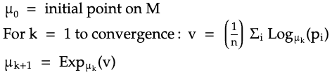
This iterative process converges to the intrinsic center, respecting the manifold’s geometry rather than cutting through it.

Projecting to the Tangent Space

Once we have μ, we project each manifold point pᵢ into the tangent space T_μM using the logarithmic map:

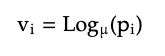
This operation is manifold-specific. For the 2-sphere S², the logarithmic map uses spherical trigonometry. For rotation groups SO(3), it employs matrix logarithms. For symmetric positive-definite matrices SPD, it leverages affine-invariant geometry. The key insight is that geodesics through μ become straight lines through the origin in T_μM.

Establishing Local Coordinates

The tangent space T_μM is a vector space with dimension d = dim(M). We construct an orthonormal basis {e₁, e₂, …, eₐ} and express each tangent vector in these coordinates. This representation is critical; all subsequent interpolation occurs in this flat, Euclidean space, where our intuitions about smoothness, derivatives, and integration directly apply.

Such a projection is universal. Whether working with 3D rotations (d=3), spherical data (d=2), or 6×6 covariance matrices (d=21), the tangent space provides a consistent framework for smooth interpolation.

Step 2: Apply Logistic Blending to Derivative Transitions

This is where the method diverges from existing approaches. Rather than constructing smooth position curves directly, we focus on ensuring smooth derivative transitions.

The Windowed Smoothstep Function

For each segment between points xᵢ and xᵢ₊₁ in tangent space, we introduce a normalized parameter τ ∈ [-1, 1] defined by arc-length. This allows for connections of points that would have otherwise not been possible when operating in the Cartesian plane.

However, this parameterization is not the central focus of the interpolation method, and for better recognizability of the well-known functions, I will walk through the method simply with respect to x and y, and briefly describe the process afterwards.

The core functions of our method are the sigmoid function and polynomial representations of the sigmoid:

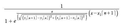
Sigmoid Function (Logistic Smoothstep)

Nested conditional statement representing specific applications of the polynomial representations of the smoothstep, for increasing differentiability

These functions contain two critical parameters:

Parameter a controls transition sharpness. Small values produce smooth, gradual blending. Large values approach piecewise-linear behavior, reducing overshoot but sacrificing some smoothness. This provides intuitive, single-parameter control over the interpolation character, unlike methods requiring separate tension and bias adjustments.

Parameter c governs continuity order. Setting c=0 ensures C¹ continuity (smooth velocity). Setting c=0.5 guarantees C² continuity (smooth acceleration). Setting c=1 achieves C³ continuity (smooth jerk). This parametric control over higher-order derivatives is crucial for optimization stability, research endeavours.

Tangent Plane Interpolation Methodology

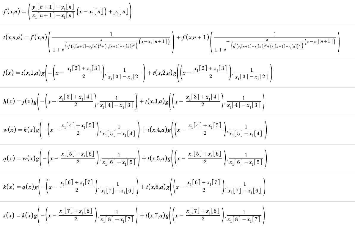
Interpolation system for 9 points

To understand how the curve is constructed, it helps to begin with the most basic component, the function f(x, n); it represents the straight line connecting consecutive points in the dataset. Each segment links the pair (xₙ, yₙ) to (xₙ₊₁, yₙ₊₁). By itself, this produces a piecewise linear path that is locally accurate but lacks smooth global behavior.

The central element of the method is the function t(x, n, a). Instead of interpolating between two points, this function operates across three consecutive samples. It passes exactly through the middle point while using the two surrounding points to determine curvature. The parameter, a controls how close the curve remains to a straight line. Larger a-values produce nearly linear behavior, while smaller values introduce stronger curvature and potential overshoot. This single parameter provides direct and intuitive control over the shape of the curve without the need for additional tuning variables.

All below interpolation functions are constructed as shifted combinations of t(x, n, a). Each of these terms is active only within a specific local region, which is enforced using the polynomial smoothstep function. A key property of the polynomial smoothstep is that it reaches the values 0 and 1 exactly rather than approaching them asymptotically. Its steepness is determined by the spacing between neighboring points, allowing transitions to occur precisely at the control points. Because of this, additional segments can be introduced without accumulating numerical error across the curve, switching from regression to interpolation.

This construction has an important consequence. Since t(x, n, a) depends on f(x, n + 1), each interpolated segment implicitly references a forward point in the dataset. As a result, the interpolation cannot naturally pass through the final point because doing so would require a point beyond the available data. The same limitation applies at the beginning of the curve, where earlier context is missing.

This behavior reflects a fundamental property of derivative based smoothing methods. Curvature cannot be defined without surrounding information. To address this, auxiliary endpoints are introduced. These additional points extend the dataset slightly beyond its true boundaries, allowing the interpolation to resolve cleanly at the ends. The presence of auxiliary endpoints also enables explicit control over endpoint behavior. By choosing them appropriately, the curve can be constructed so that its second derivative vanishes at the boundaries, producing a natural and smooth transition into and out of the interpolated region.

The resulting interpolation is smooth across the entire domain, accurate within each local segment, and stable as additional points are added. These properties become especially important when the curve represents evolving dynamics rather than static geometry, such as learning trajectories constrained to a manifold.

Let’s now apply the method to some specific Cartesian and Arc-length Parameterized examples:

Cartesian:

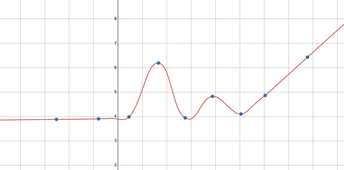
a=6.3 (moderate linearity), c=1 (C³ continuous)

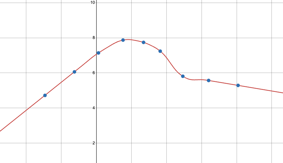
a=3 (curved behavior), c=0.5 (C² continuous)

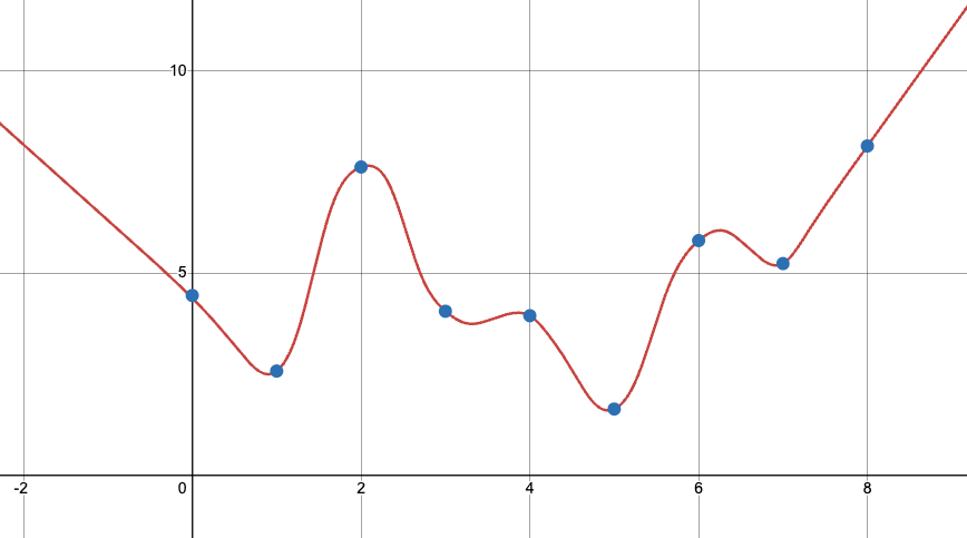
a=10 (moderate linearity), c=1 (C³ continuous)

Arc-length Parametrized:

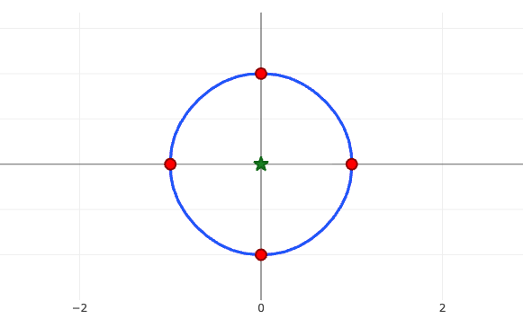
a=0.1 (substantial curvature/overshoot), c=3 (C³ continuous)

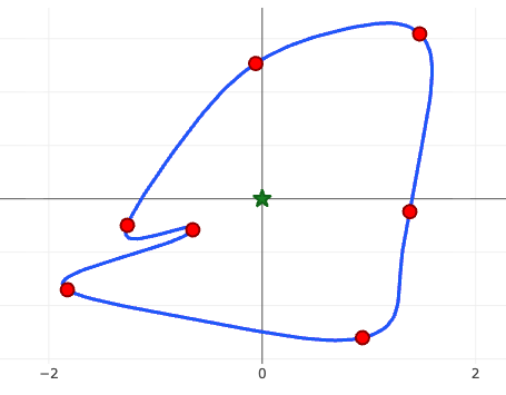
a=1 (curved with low overshoot), c=0.5 (C² continuous)

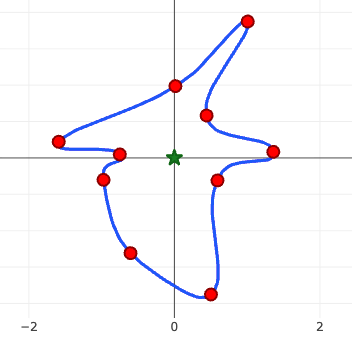
a=1.3 (curved, low overshoot, slight linearity visible), c=1 (C³ continuous)

Step 3: Map Back to Manifold via Exponential Map

The final step returns our smooth tangent space curve to the manifold, automatically enforcing all geometric constraints.

The Exponential Map

For each interpolated tangent vector vᵢₙₜₑᵣₚ(t), we apply the exponential map:

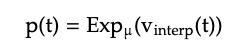
This operation is the inverse of the logarithmic map from Step 1. It takes straight lines in the tangent space and curves them along geodesics on the manifold. The specific form depends on the manifold structure:

S² (unit sphere): Exp_μ(v) = cos(‖v‖)·μ + sin(‖v‖)·(v/‖v‖)

SO(3) (rotation matrices): Exp_R(Ω) = R · exp(Ω̂) using matrix exponential

SPD (positive-definite matrices): Exp_P(V) = P^(1/2) exp(P^(-1/2)VP^(-1/2)) P^(1/2) with affine-invariant metric

Hyperbolic spaces: Exp_p(v) = cosh(‖v‖)·p + sinh(‖v‖)·(v/‖v‖) for Poincaré model

Grassmannians and Stiefel manifolds: QR-based or Cayley transform exponentials

Automatic Constraint Satisfaction

The exponential map’s mathematical structure guarantees that the resulting curve satisfies all manifold constraints. For spheres, unit norm is preserved. For rotation matrices, orthogonality and unit determinant are maintained. For SPD matrices, symmetry and positive-definiteness are enforced. No projection, normalization, or correction step is required, the geometry does the work.

This is fundamentally different from other approaches that interpolate in ambient space and project back. Those methods accumulate error and can produce discontinuities when the projection operation varies sharply. By working through the tangent space and exponential map, we guarantee that every point on our interpolated curve genuinely belongs to the manifold.

Generating the Parametrized Curve

To produce the complete interpolated trajectory, we sample uniformly across the arc length parameter domain [t₀, tₙ]. For each sample point t, we determine which segment contains it, compute the normalized local parameter τ, then evaluate vᵢₙₜₑᵣₚ(τ) in tangent space, and map to the manifold via Exp_μ. The result is a smooth curve that flows naturally along the manifold’s surface, respecting its intrinsic geometry at every point.

Universal Applicability Across Manifolds

This three-step framework is not tied to any specific manifold. It works identically whether we’re interpolating on 2-spheres for directional data, rotation groups for robotics, SPD matrices for covariance estimation, or Grassmannians for subspace learning. The only requirements are:

A logarithmic map Log_μ: M → T_μM An exponential map Exp_μ: T_μM → M A Fréchet mean computation algorithm

These operations exist for every Riemannian manifold encountered in machine learning applications. Even exotic manifolds like fixed-rank matrix spaces, shape manifolds, or product manifolds can leverage this framework. The interpolation logic in Step 2 never changes, it operates purely in the flat tangent space, independent of the manifold’s global structure.

This universality is crucial for AI systems. As machine learning increasingly employs geometric structure, from orthogonal neural network layers (Stiefel manifolds) to covariance adaptation (SPD manifolds) to hierarchical embeddings (hyperbolic spaces), having a single interpolation framework that handles all cases seamlessly reduces implementation complexity and ensures consistent behavior across different geometric domains.

Computational Advantages

The method’s structure provides several practical benefits for integration into training pipelines:

Efficiency:

Once tangent vectors are computed, interpolation reduces to evaluating a logistic function, performing scalar multiplication, and applying the exponential map. These operations are fast compared to iterative projection schemes.

Stability:

Working in tangent space avoids the numerical issues that plague repeated projection operations, particularly on high-curvature manifolds where small errors accumulate rapidly.

Parallelizability:

Each segment can be processed independently, enabling efficient vectorization and GPU acceleration critical for large-scale optimization.

Differentiability:

The entire pipeline is differentiable end-to-end. Gradients flow cleanly from loss functions through the exponential map, tangent space operations, and back to parameters. This makes the method compatible with automatic differentiation frameworks like PyTorch and JAX.

Scalability:

Computational complexity grows with the tangent space dimension d = dim(M), not with ambient space dimension. For SPD(n) matrices embedded in n×n space, we work in d = n(n+1)/2 dimensions rather than n², a significant reduction for large n.

These properties make the method practical for real training loops where thousands or millions of parameter updates occur. The overhead is minimal, but the stability benefits compound over the course of optimization, potentially reducing the total number of iterations needed for convergence.

Why This Matters for AI Going Forward

If LLMs, RL policy networks, or low-rank finetuned models could update smoothly, we might see:

• Faster convergence in unstable regions,
• Better generalization from continuous parameter motion,
• Safer training for autonomous agents,
• Improved long-run reliability.

The research isn’t only about interpolation. It’s about teaching AI to learn like a river, not a bouncing ball.

The Barriers & Next Steps

To move toward real-world application, I need to:

1. Benchmark performance against SLERP, SQUAD, SENO 2. Extend to high-dimensional manifolds (SPD, SE(3)) 3. Apply while training known AI models, and compare behavior (CLIP, NucleusDiff, STELLA, and ResNet-(18, 20, 56) ) 4. Develop a complete framework and publish as open research

This work is foundational, but the trajectory is promising,

AI shouldn’t just learn correctly, it should learn smoothly.