Modeling Levels in Vehicle Vertical Dynamics

When engineers try to understand how a vehicle responds to road disturbances, they rarely start with the most complex simulation available.

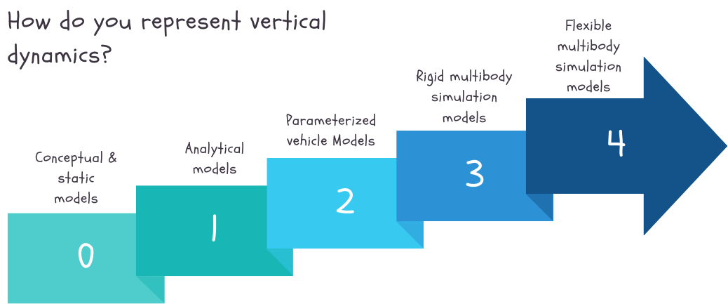
Instead, engineers move through layers of modeling fidelity.

Model fidelity describes the degree to which a model represents reality. It measures how “faithful” the model’s behavior and outcomes are to the actual physical system.

At one extreme, the vehicle may be reduced to a simple mass connected to a spring and a damper. At the other end is the full multibody simulation (MBS), where every suspension link, bushing and joint can be represented explicitly.

The choice of modelling approach is often influenced by factors such as computational effort, software licensing costs, and the existing engineering toolchain. But from an engineering perspective, the difference lies in what question the engineer is trying to answer.

• A simple model might reveal the dominant vibration modes of the vehicle body.
• A more detailed system model can represent nonlinear damper behavior and realistic tire forces.
• A full MBS can capture how suspension geometry redistributes forces through individual links and bushings.

Interpreted from a vertical dynamics perspective:

• Analytical models capture the dominant modal behavior of the vehicle.
• Parameterized system models capture nonlinear force behavior and realistic tire-road interaction.
• MBS captures geometric coupling effects within the suspension.

Understanding when to use each level is an important skill for engineers working on ride comfort, suspension design, or vehicle simulation.

Note regarding the abbreviations here: DOF — Degrees Of Freedom, MF — Magic Formula, ODE — Ordinary Differential Equation, DAE — Differential Algebraic Equation, SiL — Simulation-in-Loop, HiL — Hardware-in-Loop.

The modelling approaches shown above do not simply differ in complexity. Each approach exposes different physical mechanisms of the suspension system and supports different stages of engineering analysis.

Level 0 — Conceptual and Static Models

Before running any dynamic simulation, engineers often start with something much simpler: basic static calculations.

At this stage, the suspension is not treated as a dynamic system. Instead, it is analyzed using static equilibrium and stiffness relationships.

Typical questions at this level include:

• What spring stiffness is required to support the vehicle?
• What will be the static suspension deflection?
• What ride frequency will the vehicle body have?

These questions can often be answered using simple relationships such as the well-known approximation of the ride frequency:

where k is the effective suspension stiffness and m is the sprung mass.

Although extremely simple, these calculations provide valuable insight into basic vertical behavior of the vehicle. For example, passenger cars typically target ride frequencies in the range of 1–1.5 Hz, which sport vehicles often use higher values.

Because these models involve only algebraic equations, they can be evaluated almost instantly and are frequently used during the early concept phase of suspension design.

However, static models cannot capture transient behavior, damping effects, or the response of the vehicle to road disturbances. For that, engineers must move to dynamic models.

This stage is sometimes not considered a “model” in the strict sense, but it represents the starting point of many suspension design calculations.

Level 1 — Lumped-Parameter Analytical Models

Next, the vehicle is treated as a dynamic system composed of lumped masses connected by springs, dampers and optionally external forces (like actuators).

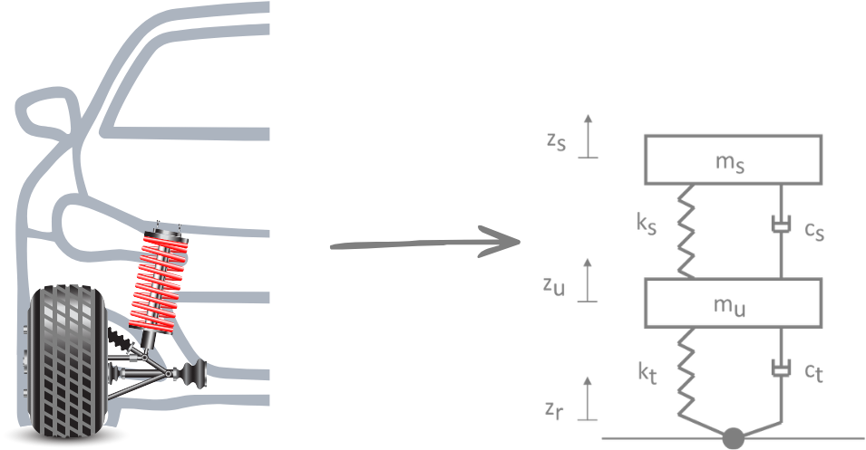
Physical Model → Linear Quarter Car Model

Instead of analyzing only static equilibrium, the system is now described using equations of motion that govern how the vehicle responds to road disturbances over time.

The most common representations include:

• Quarter-car model (2 DOF)
• Half-car model (4 DOF)
• Full-vehicle ride model (7 DOF)

In some ride comfort studies, additional degrees of freedom may be introduced to represent seat dynamics or simplified human body models, allowing the analysis to capture how vibrations are transmitted to the occupant.

These models represent the vehicle using a small number of lumped masses (LM), typically including:

• the sprung mass (vehicle body or mass supported by the suspension system)
• the unsprung mass (wheel assembly or mass not supported by the suspension system)

connected through:

• suspension springs
• dampers
• actuators (optional)
• tire stiffness and damping elements

Unlike MBS, the suspension geometry is not represented explicitly. Instead the mechanical behavior of the suspension is reduced to equivalent parameters such as stiffness and damping coefficients.

Mathematical Representation

Lumped-parameter models are typically described by systems of ODEs. For example, the classic linear quarter-car model can be written as:

Although these models are often presented with linear springs and dampers, nonlinear force elements can easily be introduced. For example, spring or damper forces may be represented using nonlinear functions or lookup tables. The primary limitation of these models is therefore not force nonlinearity, but the absence of explicit suspension geometry.

What These Models Capture

Despite their simplicity, lumped-parameter models reveal several key characteristics of vertical vehicle dynamics:

• bounce mode of the vehicle body
• pitch and roll modes (in half-car and full-car models)
• ride frequency and damping behavior
• interaction between sprung and unsprung masses

Because the system is represented by only a few degrees of freedom, the resulting dynamics are often easy to interpret in terms of modal behavior.

What These Models Do Not Capture

The simplicity of these models also introduces limitations. Analytical ride models typically do not represent:

• suspension kinematic nonlinearities
• camber variation and link geometry effects
• detailed bushing compliance
• load redistribution through suspension links

All suspension behavior is effectively reduced to equivalent stiffness and damping parameters.

Typical Engineering Use

Because of their simplicity and computational efficiency, lumped-parameter models are widely used for:

• control algorithm development
• parameter sensitivity studies
• conceptual understanding of ride dynamics
• early suspension design studies

In many cases, these models serve as the starting point for understanding the dominant vibration behavior of the vehicle before more complex simulations are introduced.

Level 2 — Parameterized Full-Vehicle Models

Typical Examples: CarSim, CarMaker and veDyna

As the analysis moves beyond simple ride modes, engineers often need to study how the entire vehicle responds to road excitation. At this stage, interactions between multiple subsystems become important, including the suspension, tires, and vehicle body motions.

Analytical models can represent some of these effects, but managing many interacting nonlinear components quickly becomes difficult when the system is described using only a small number of degrees of freedom.

To address this, engineers often use parameterized vehicle models.

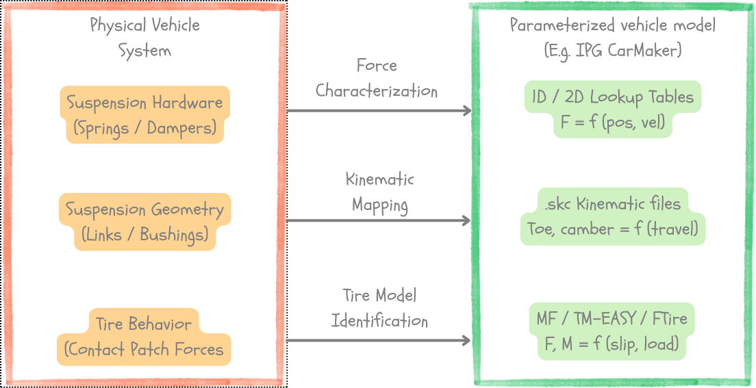
Representation of physical vehicle subsystems in a parameterized vehicle model. This approach enables efficient full-vehicle simulations used in tools such as CarMaker.

In this modelling approach, the vehicle is represented using a structured dynamic model, while many suspension effects are embedded through parameterized relationships or lookup tables (LT) derived from suspension geometry, measurements, or higher-fidelity simulations.

Unlike multibody simulations, the suspension links are not represented explicitly. Instead, their behavior is captured through predefined kinematic and compliance relationships.

These models can represent vehicle-level dynamic behavior while keeping the model computationally manageable.

Mathematical Representation

Parameterized vehicle models are typically formulated as a structured system of ordinary differential equations (ODEs) describing the motion of the vehicle body and wheel masses.

The generalized form of the equations can be written as

where:

• q represents the generalized coordinates (vehicle body motions and wheel motions)
• M(q) is the mass matrix
• C(q,q̇) represents the inertial and damping terms
• F(q,q̇) represents suspension and tire forces
• Fₑₓₜ represents external inputs such as road excitation or actuator forces

In this modeling approach, suspension behavior is not computed from explicit link geometry. Instead, suspension effects are embedded through parameterized relationships, such as:

• lookup tables derived from suspension kinematic analysis
• predefined functions describing wheel travel vs. suspension forces
• lumped compliance models for bushings and mounts

Because the suspension geometry is not solved using constraint equations, the system remains a pure ODE problem.

This has an important computational consequence — the model can be solved using standard numerical integration methods like:

• explicit Runge-Kutta methods
• fixed-step integrators used in real-time simulations
• variable-step solvers for offline analysis

Since no constraint Jacobians or algebraic constraints need to be solved, the numerical system remains comparatively lightweight. This is one of the main reasons why parameterized vehicle models are often capable of real-time execution, making them suitable for Software-in-the-Loop and Hardware-in-the-Loop environments.

What These Models Capture

Compared to analytical ride models, parameterized vehicle models can capture additional aspects of vehicle behavior, including:

• nonlinear suspension characteristics
• realistic tire behavior
• coupling between vehicle motions (bounce, pitch, roll)
• vehicle response to road profile excitation
• simplified suspension kinematic effects through parameterized relationships

This allows engineers to study vehicle-level ride behavior under more realistic conditions.

What These Models Do Not Capture

Despite their capabilities, these models still simplify several aspects of suspension behavior.

In particular, they do not resolve:

• exact force paths through individual suspension links
• detailed joint-level load distribution
• local deformation of bushings
• structural flexibility of suspension components (unless externally coupled)

Computational Behavior

One of the main advantages of parameterized vehicle models is their computational efficiency.

Typical characteristics include:

• real-time capable simulations
• suitable for Software-in-the-Loop (SiL) environments
• suitable for Hardware-in-the-Loop (HiL) testing

Typical Engineering Use

Parameterized vehicle models are commonly used for:

• system integration studies
• ADAS validation
• suspension tuning studies
• controller validation within a vehicle simulation environment

They therefore represent an important modelling layer between analytical ride models and constraint-based multibody simulations.

Level 3 — Constraint-Based Rigid MBS

Typical Examples: Adams, Simpack, RecurDyn and Dymola

When engineers want to understand how forces propagate through the actual suspension structure, parameterized vehicle models are often no longer sufficient. At this point the geometry of the suspension itself becomes important.

In multibody simulation, the vehicle suspension is no longer approximated using equivalent parameters or lookup tables. Instead, the suspension is represented as a mechanical assembly composed of rigid bodies connected through joints and constraints.

Each suspension component — such as control arms, knuckles, wheel carriers and subframes — is represented explicitly, and the motion of the system is determined by solving the equations that enforce the kinematic constraints between these bodies.

Because the mechanical structure is represented directly, this modelling approach allows engineers to analyze the true geometric behavior of the suspension system.

Typical joints used in vehicle suspension models include:

• revolute joints
• spherical joints
• translational joints
• compliant bushings

Together, these constraints define how the suspension can move relative to the vehicle body.

Mathematical Representation

Unlike lumped-parameter or parameterized vehicle models, multibody simulations are typically described using differential–algebraic equations (DAEs) rather than pure ordinary differential equations.

The equations of motion can be expressed in the form

where

• q represents the generalized coordinates of all bodies
• M(q) is the system mass matrix
• Q represents applied forces such as springs, dampers and tire forces
• Φ(q) represents the constraint equations describing the joints
• λ represents the constraint forces enforced through Lagrange multipliers

These equations simultaneously enforce:

• dynamic motion of the bodies
• kinematic constraints imposed by the joints

Because both the dynamic motion and the joint constraints must be solved simultaneously, multibody simulation tools typically employ implicit numerical integration methods such as backward differentiation formulas (BDF) together with constraint stabilization techniques like Baumgarte stabilization.

What These Models Capture

Constraint-based multibody simulations allow engineers to analyze several phenomena that cannot be represented accurately in lower-fidelity models:

• exact suspension kinematics
• force distribution through suspension links
• wheel camber and toe variation during suspension travel
• load transfer through suspension geometry
• joint reaction forces and bushing loads

Because the suspension geometry is explicitly represented, these models are particularly valuable for kinematics and compliance (K&C) analysis.

Computational Behavior

The increased level of detail in multibody simulations introduces a significantly higher computational cost.

Compared with parameterized vehicle models, MBS simulations are typically:

• computationally intensive
• unsuitable for real-time simulation in most cases
• primarily used for offline engineering analysis

However, they provide the highest level of physical fidelity available in vehicle dynamics simulation before prototype testing.

Typical Engineering Use

Constraint-based multibody simulations are widely used for:

• suspension kinematics and compliance analysis
• load distribution studies within suspension components
• detailed ride and handling investigations
• suspension design validation prior to prototype testing

Level 4 — Flexible Multibody Simulation

The rigid-body assumption used in classical multibody simulation is sufficient for many vehicle dynamics studies. However, when structural flexibility begins to influence the dynamic behavior of the suspension system, the rigid-body approximation becomes insufficient.

At this stage, the suspension components themselves must be allowed to deform under load.

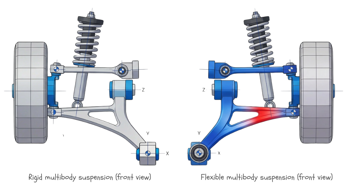
Illustration generated using AI (Perplexity)

Flexible multibody simulation extends rigid multibody models by replacing selected rigid components with flexible bodies derived from finite element models. These flexible bodies capture structural deformation while still participating in the multibody dynamic system.

Because of this, flexible multibody models combine multibody dynamics and structural mechanics within a single simulation framework.

In flexible multibody simulations, certain suspension components such as:

• control arms
• subframes
• wheel carriers
• chassis attachment structures

are represented using reduced-order flexible bodies obtained from finite element models.

The deformation behavior of these components is typically represented using modal reduction techniques, allowing the flexible structure to be integrated into the multibody simulation without solving the full finite element problem at every time step.

Mathematical Representation

Flexible multibody models extend this formulation by allowing certain components to deform. Additional coordinates are introduced to represent elastic deformation.

A simplified form of the equations becomes:

where

• Kq represents internal elastic forces arising from structural deformation
• q now includes both rigid body motion and elastic deformation coordinates

This additional stiffness term allows the simulation to capture structural compliance effects in suspension components.

The equations of motion of flexible multibody systems form a set of coupled differential–algebraic equations (DAEs) that include both rigid body motion and structural deformation.

Because flexible components introduce additional stiffness into the system, the resulting equations are often numerically stiff.

To ensure stable time integration, multibody simulation tools typically employ implicit numerical integration methods, such as:

• Backward Differentiation Formula (BDF) methods
• Generalized-α method
• Newmark-β method

These integrators allow the solver to handle the stiff dynamic behaviour introduced by flexible components while simultaneously enforcing the constraint equations of the multibody system.

The increased numerical complexity of flexible multibody models is one of the reasons why such simulations are typically used for detailed offline analysis rather than real-time vehicle simulation.

What These Models Capture

Flexible multibody simulations allow engineers to capture phenomena such as:

• deformation of suspension arms under load
• subframe flexibility
• compliance of lightweight suspension components
• coupling between structural vibration and vehicle dynamics

These effects become particularly relevant when lightweight structures or compliant components significantly influence the suspension behavior.

Computational Behavior

Because flexible bodies introduce additional degrees of freedom, these simulations are typically:

• significantly more computationally demanding
• unsuitable for real-time simulation

Typical Engineering Use

Flexible multibody simulations are commonly used for:

• structural compliance studies
• lightweight suspension design validation
• investigation of structural vibration effects
• correlation between multibody and finite element models

Closing Remark

The modelling hierarchy discussed here was illustrated using examples from vertical vehicle dynamics, where ride comfort and suspension behavior are often studied using different levels of model fidelity.

However, the same modelling philosophy applies across many other areas of vehicle dynamics. Engineers working on handling, braking, powertrain dynamics, or ADAS simulation frequently move between similar modelling layers depending on the question being investigated.

Simple analytical models may provide intuition about dominant system behavior, parameterized vehicle models allow efficient full-vehicle simulations, and multibody simulations reveal detailed mechanical interactions within the suspension structure. Flexible multibody models further extend this framework by capturing structural deformation effects.

In practice, engineers rarely rely on a single modelling approach. Instead, they move between these levels of fidelity to balance physical insight, computational efficiency, and simulation realism.

While this article focused on vertical dynamics, the underlying modelling hierarchy is broadly applicable to vehicle dynamics simulation as a whole.