How Do Modern LLMs Cheat the Scaling Laws? (In a Good Way).

If you’ve been following LLMs closely, you’ve probably noticed a pattern: parameter counts explode, GPU bills explode, but inference still needs to be fast enough to power your chat window.

Mixture of Experts (MoE) architectures are one of the clever hacks that let you have “trillion-parameter” models without paying a trillion-parameter compute bill on every token.

I want to talk about everything from the intuition to the math, and then into the real engineering workflow of MoE in production systems like GShard, Switch Transformer, and Expert Choice routing.

Why MoE Exists

Dense transformers have a simple rule: every token passes through the same set of parameters in every layer. That makes them conceptually clean, but it also means your compute cost scales linearly with the number of parameters you add.

Empirically, scaling laws show that bigger models usually perform better, but training a dense 11 trillion-parameter model is financially and operationally painful. MoE changes the game by making only a small subset of the parameters “active” per token.

The core idea is conditional computation: instead of using one giant generalist network, you build many specialist “experts” and learn a router (gating network) that decides which experts each token should consult.

Analogy

Think of this in the case of a hospital:

• You don’t send every patient to every department.
• A triage nurse quickly routes each patient to 1–2 specialists.
• Most capacity sits idle for any given patient, but the total capacity of the hospital is huge.

The triage nurse is your gating network. The departments are experts. The full hospital is the MoE layer.

The goal during training is for the router to learn meaningful specialization: some experts become great at code, some at long-tail languages, some at math, etc., while still keeping the system balanced and trainable.

Why Dense Scaling Laws Break Down

Before understanding why MoE is clever, I think it’s important to understand exactly what it’s cheating against: the Chinchilla scaling laws.

In 2022, DeepMind’s Hoffmann et al. published a landmark paper (colloquially called “Chinchilla”) that changed how we think about training large language models optimally. The core finding was that for a given compute budget CCC, the optimal dense model allocates roughly equal scaling between model parameters NNN and training tokens DDD, with the rule of thumb being approximately 20 tokens per parameter.

To put it formally, compute scales as:

C ≈ 6ND

where the factor of 6 accounts for the forward and backward pass FLOPs per parameter per token. This meant that GPT-3 (175B parameters, trained on ~300B tokens) was dramatically undertrained by Chinchilla’s standards. You’d need roughly 3.5 trillion tokens to optimally train a 175B model.

The practical implication was clear: if you want a smarter model under a fixed compute budget, you’re often better off training a smaller model for longer than a massive model for fewer steps. Chinchilla-70B, trained on 1.4 trillion tokens, outperformed Gopher (280B) and GPT-3 (175B) on most benchmarks at a fraction of the inference cost.

The Chinchilla Wall

These laws are powerful, but they assume a dense architecture where every parameter is active for every token, and compute scales linearly with model size. Under this model, doubling parameters means doubling FLOPs per token at inference, forever. You eventually hit a wall: a 1-trillion-parameter dense model may be theoretically optimal for some tasks, but the per-token inference cost becomes financially and operationally brutal. Serving a trillion-parameter dense model at scale would require enormous GPU clusters just to keep latency acceptable.

This is exactly the constraint MoE sidesteps. The Chinchilla framework gives you the optimal training recipe for dense models, but it has no clean answer for: “What if I want 1T parameters of capacity but only want to pay for 13B parameters of compute per token?” That question requires a different scaling framework altogether.

MoE Scaling Laws

Recent research (including DeepMind’s joint MoE scaling laws, 2025) has begun formalizing how MoE models scale differently. The key insight is that MoE decouples two quantities that are fused in dense models:

• Total parameters Ntotal​=E×Nexpert​ — the “capacity” of the model
• Active parameters per token Nactive​=k×Nexpert​ — the actual compute cost.

In a dense model, Ntotal​=Nactive​ always. In a sparse MoE model with EE experts and top-kk routing, you get:

Nactive/Ntotal = k/E

For Mixtral 8×7B with k=2k=2k=2, this ratio is 2/8 = 25%. For models like GPT-4 and Gemini Ultra, which are widely believed to use MoE with many more experts, this ratio is estimated to be somewhere in the 5–15% range. This means you’re activating a small fraction of total capacity per token.

This is why MoE “cheats” the Chinchilla scaling laws in a good way: you can build a model with the capacity of a trillion-parameter dense network while paying the compute cost of a much smaller one. Chinchilla tells you the optimal training recipe for a given FLOP budget on dense models. MoE says: “What if we stretch that FLOP budget across far more parameters by making most of them conditionally inactive?”

The tradeoff is that Chinchilla’s optimal token-to-parameter ratio no longer applies cleanly. Emerging MoE-specific scaling research suggests the optimal activation ratio decreases as models scale. At very large scales, activating ~7–8% of experts may be near-optimal. However, the exact Chinchilla-equivalent for MoE is still an active area of research as of 2025–2026.

With that tension in mind, let’s look at exactly how MoE restructures the FFN to make conditional compute possible.

Dense Layers To Experts

Take the standard transformer feedforward (FFN) block: a big MLP applied independently to each token. In a dense model, that FFN has one set of weights shared across all tokens and all positions in that layer.

In an MoE layer, you replace that single MLP with EEE different MLPs, each one an “expert,” and then let a small router decide which experts each token should visit. Intuitively, instead of one generic “brain,” you now have a panel of specialists, and each token gets routed to a few that are likely to understand it best.

The Core MoE Equation

Formally, an MoE layer with experts E1​,…,EE​ and gating weights w1​,…,wE​ produces:

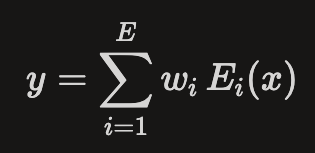
The gating network computes a score vector g(x)g(x)g(x), usually normalized with softmax, and then sparsifies it so that only the top-kkk entries remain non-zero:

gi(x)={softmax(Wgx)iif i∈top-k(Wgx)0otherwiseg_i(x) = \begin{cases} \text{softmax}(W_g x)_i & \text{if } i \in \text{top-}k(W_g x) \ 0 & \text{otherwise} \end{cases}gi​(x)={softmax(Wg​x)i​0​if i∈top-k(Wg​x)otherwise​

This means only the top-k experts actually run for a given token, and their outputs are linearly combined with the corresponding non-zero gate weights to produce the final output of the MoE layer. When k≪E, total parameters scale with E but per-token compute is dominated by only those k experts, which is the key trick behind MoE’s scalability.

Sparse Activation and Conditional Compute

The defining feature of modern MoE for LLMs is sparse activation: for each token, only a small subset of experts do any work. This is different from the original “dense” MoE formulations where every expert contributed, just with different weights, which kept compute scaling linearly with the number of experts.

Sparse MoE uses a router to compute affinities between tokens and experts, selects the top-kkk experts (often k=1k=1k=1 or k=2k=2k=2), and zeroes out the rest, drastically reducing the number of MLPs evaluated per token. Architectures like Switch Transformer (top-1 routing), GShard (top-2), GLaM, and V-MoE show that you can get better quality-to-compute tradeoffs with sparse MoE layers than with purely dense transformers of the same FLOP budget.

Who Chooses Whom?

Routing (deciding which expert handles which token) is the core MoE design problem. At a high level, there are three broad families of routing strategies you’ll see in the literature:

• Token-choice routing: tokens pick their experts, e.g., “sparsely gated” MoE and Switch-style top-kkk gating.
• Expert-choice routing: experts pick their tokens, e.g., Expert Choice Routing.
• Global assignment: a separate mechanism (like a matching algorithm) assigns token-expert pairs under constraints.

In token-choice routing, the router looks at each token’s representation, scores all experts, and picks the top-kkk experts for that token, which is how Switch Transformer, GLaM, and many modern MoE LLMs operate. Expert-choice flips this: each expert looks at a pool of tokens and chooses which ones to handle, which can improve load balancing and training efficiency when combined with good selection heuristics.

Global assignment methods treat routing like a constrained optimization problem (e.g., variations of linear assignment or k-means), but are mostly used in research prototypes rather than large production LLMs due to complexity.

The Life Of A Token In An MoE Layer

On a forward pass, a typical Transformer+MoE layer does roughly the following:

1. The router takes the token embeddings for the current layer, applies a small linear (or MLP) projection, and computes logits over the EEE experts for each token.
2. A softmax converts logits to probabilities, and the router selects the top-kkk experts per token, often with some stochasticity or noise added during training.
3. Tokens are bucketed by their chosen experts, and an all-to-all communication step shuffles token embeddings across GPUs so each expert sees the tokens assigned to it.
4. Each expert runs its own feedforward MLP on the tokens it received, in parallel across GPUs.
5. Another all-to-all shuffles the expert outputs back to their original token positions, and the router recombines them using the corresponding gate weights, producing a single tensor that replaces the dense FFN output.

All the ugly systems work is in steps 3 and 5: the all-to-all collectives over potentially huge token batches and many GPUs, which can easily become the latency bottleneck if the implementation is not tuned.

Capacity, Overflow, And The “Capacity Factor”

In practice, you cannot let any expert receive an unbounded number of tokens per batch, or you’ll blow up memory and latency on that expert’s GPU. MoE implementations therefore define a capacity per expert (the maximum number of tokens it will process in a batch), computed as:

Capacity=⌈tokens per batchE×capacity factor⌉\text{Capacity} = \left\lceil \frac{\text{tokens per batch}}{E} \times \text{capacity factor} \right\rceilCapacity=⌈Etokens per batch​×capacity factor⌉

If a router tries to send more tokens to an expert than its capacity, those extra tokens “overflow.”

Different systems make different choices for overflow tokens: some drop them entirely (token dropping), some reroute them to backup experts, and some attempt “dropless” MoE where routing and capacity are tuned so that almost no token is dropped. The capacity factor is a key hyperparameter: low capacity factors improve efficiency but increase overflow risk, while high capacity factors reduce overflow but increase memory and communication cost.

Expert Collapse And Load Imbalance

Left to itself, a naive router tends to fall in love with a few experts and ignore the rest. This “expert collapse” means some experts become over-specialized and overloaded, while many never get enough gradient signal to learn anything useful.

To prevent this, modern MoE models add auxiliary losses that encourage balanced routing, such as penalizing high variance in the fraction of tokens assigned to each expert and encouraging higher router entropy. Google’s sparsely-gated MoE and later models like Switch Transformer rely on such load-balancing losses to keep experts active and avoid under-training or over-training subsets of experts.

Expert Choice Routing goes further by letting experts choose tokens under constraints that inherently encourage better load balance, resulting in more than 2× faster convergence in an 8B/64E setup compared to earlier GShard and Switch top-kkk routing. That result highlights a key MoE theme: most of the gains don’t come from just “more experts,” but from routing strategies that keep those experts meaningfully busy without overloading any of them.

Real Systems: Switch, GLaM, V-MoE, Expert Choice

The modern MoE story in LLMs really took off with Google’s sparsely-gated MoE layers and the Switch Transformer. Switch simplifies routing by sending each token to only its top-1 expert (k=1k=1k=1) instead of top-2 or more, which significantly reduces communication and routing overhead while still benefiting from conditional computation.

GLaM scales MoE to large language models by using top-kkk routing with many experts per layer and shows better scaling than dense transformers on NLP benchmarks at comparable compute budgets. V-MoE applies a similar sparsely-gated MoE idea in vision transformers, routing image patches to experts and showing competitive performance-to-compute tradeoffs on large-scale vision tasks.

Expert Choice Routing, proposed by Google researchers, introduces a new routing method where experts select tokens, addressing load imbalance and under-utilization issues found in earlier MoE designs. Experiments show that at the 8B/64E scale, Expert Choice yields more than 2× faster convergence in training perplexity compared to GShard top-2 and Switch-style gating, while also scaling well as the number of experts or expert capacity increases.

Mixtral, DeepSeek, And MoE In Today’s LLMs

Recent open and commercial LLMs like Mixtral “8×7B” popularized the idea of having ~47B total parameters but only a small fraction active per token, thanks to MoE layers. In these models, each MoE layer might contain eight 7B-parameter experts, but the router activates only the top-2 per token, so effective per-token compute is closer to a ~13B dense model while capacity is much higher.

DeepSeek-V2 pushes this further with fine-grained MoE: rather than 8 large experts, it uses 160 smaller experts per layer with top-6 routing, which increases routing granularity and allows the model to mix specializations more fluidly per token. This fine-grained approach, combined with shared experts that every token always passes through, stabilizes training and improves generalization. This pattern is increasingly common in production-grade MoE systems.

If you look at real deployments, MoE layers often appear only in the middle of the network, where the FFN cost dominates and routing overhead can be amortized over large batches, while attention-heavy early and late layers remain dense. This kind of partial MoE design is one of the quiet “engineering compromises” that make MoE feasible in production-scale LLMs.

Where MoE Lives Inside A Transformer

Architecturally, an MoE transformer layer replaces the usual dense FFN block with an MoE block, while keeping self-attention unchanged. The sequence becomes: attention → MoE FFN → residual + normalization, just like attention → dense FFN in a standard transformer.

Inside the MoE FFN, each expert is usually just a regular transformer-style MLP (linear → nonlinearity (e.g., GELU) → linear) with its own parameters. The router operates on the input to the FFN, sends tokens to experts, and merges outputs back into the main residual stream, making the MoE layer a drop-in replacement from the rest of the model’s perspective.

Because experts are independent MLPs, you can also vary their sizes or architectures, but most production systems keep expert architectures homogeneous to simplify implementation and improve load balancing. Heterogeneous experts are an interesting research direction but complicate the already-hard routing and capacity management story.

Training Dynamics And Regularization

Training MoE models is not just “train a transformer, but with more parameters.” You typically add an auxiliary loss term for load balancing, which nudges the router towards using all experts more evenly.

Common techniques include penalizing the squared difference between the empirical token fraction per expert and the ideal 1/E1/E1/E fraction, adding entropy regularization to the router logits, and sometimes injecting noise to the router during training to encourage exploration of underused experts. These tricks help avoid dead experts (experts that virtually never see tokens and thus never learn) and maintain gradient flow across the whole expert set.

In addition, it is typical to use careful initialization and learning rate schedules for router parameters, because the router sits on a sharp, discrete decision boundary (which experts to pick), and unstable routing can easily destabilize training early on. Some systems delay turning on sparsity (training with dense or soft routing initially and then annealing to hard top-kkk) to smooth this transition.

System-Level Pain: All-To-All, Latency, And Stragglers

From a systems perspective, MoE introduces two expensive all-to-all operations per MoE layer: dispatching tokens to experts and gathering expert outputs back. On a multi-GPU or multi-node setup, those collectives can dominate wall-clock time if not optimized, even when FLOPs look favorable on paper.

All-to-all overhead scales with the number of experts, GPUs, and tokens, and is sensitive to network topology and bandwidth, so MoE efficiency depends heavily on communication libraries and topology-aware placement. Straggler experts (GPUs that get slightly more tokens or have worse locality) can delay the entire batch, because the gather step cannot finish until all experts are done.

Practical MoE deployments use tricks like overlapping communication with computation, grouping experts on fewer devices, using hierarchical all-to-all, and tuning capacity and batch size to keep all experts similarly loaded. In many benchmarks, these engineering details determine whether MoE is actually faster than a smaller dense model at the same quality level.

When MoE Is A Bad Idea

MoE is not a free lunch, and there are cases where a well-tuned dense model wins. If your deployment scale is small (few GPUs, modest batch sizes), the all-to-all overhead and implementation complexity can outweigh the benefits of conditional computation.

Dense models also have simpler failure modes and are often easier to distill, compress, and quantize, while MoE’s conditional structure complicates quantization-aware training, distillation, and serving pipelines. On some tasks with limited diversity, the specialization benefits of experts may not show up strongly at all. In these cases you are paying routing and communication costs without gaining enough capacity-driven quality improvements.

For many teams, the sweet spot is: use MoE only once you are constrained by compute but still want to push capacity and quality, have enough scale to amortize communication overhead, and have the ML + systems engineering bandwidth to debug routing and expert-health metrics.

Conclusion: What Does This Mean For You?

If you are building or researching LLMs, MoE is essentially an architectural lens on scaling: instead of “just add more layers/heads/width,” you think “add more experts and smarter routing.” When it works, you get models like Mixtral that offer near-47B capacity behavior with ~13B-like per-token cost, and training regimes like Expert Choice that converge faster at fixed compute budgets.

The trade is that you have to care about auxiliary losses, capacity factors, router stability, all-to-all latency, and expert-health dashboards, not just validation curves. If that sounds like fun rather than overhead, MoE is one of the most powerful tools you can reach for in the current LLM scaling toolbox.