Tensor and sequence parallelism — explained with pictures

A modern LLM does not fit on a single GPU. A 70B-parameter model in bf16 needs ~140 GB just for the weights, and during training the optimizer state and gradients add another 5–10× on top of that. An 80 GB H100 is not going to cut it, and even a full 8-GPU node only buys you so much breathing room.

Data parallelism is the first tool everyone reaches for. This type of parallelism replicates the model on every device and shards the batch — fine for throughput, useless for fitting a model that is bigger than one GPU.

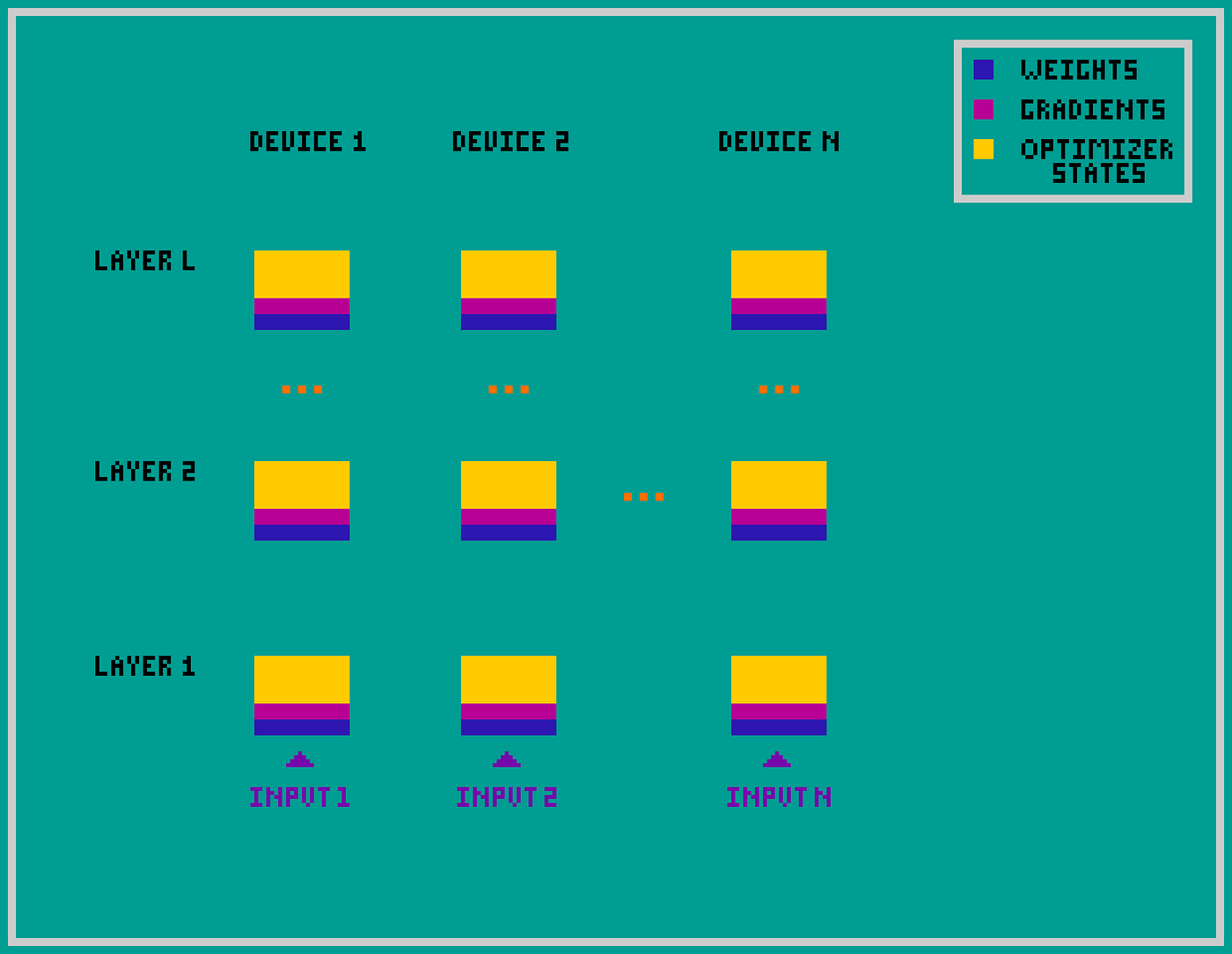
Naive data parallelism: the model is completely copied across devices

Modern training stacks fix this with FSDP (PyTorch’s Fully Sharded Data Parallel, conceptually the same thing as DeepSpeed ZeRO-3): parameters, gradients, and optimizer state are sharded across the data-parallel group, and each layer’s full weights are all-gathered on demand right before they are used, then released. Per-device weight memory drops by N and a 70B model becomes trainable on a single node.

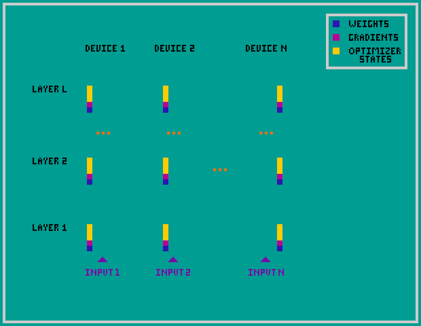
Zero-3: the model is completely distributed across several devices

So why does anyone still bother with tensor parallelism? Two reasons.

First, FSDP shards the weights, not the computation in space. At the moment a matmul runs, every device still executes the full matmul on its own slice of the batch, with the full per-layer activation tensor sitting in HBM. For wide models the activations alone overflow a single GPU, and a single matmul is bottlenecked by one device’s FLOPs and memory bandwidth — extra data-parallel replicas can’t help you finish that one matmul any faster.

Second, FSDP is awkward at inference. Gathering every layer’s weights once per generated token is a latency disaster. Production inference engines almost universally reach for tensor parallelism instead — it shards both the weights and the work, so per-token latency goes down with more devices.

The two techniques in this post all split the model across space rather than time, and they apply equally to training and inference:

• Tensor parallelism (TP) splits the weight matrices across devices, so every matmul is sharded and runs in parallel.
• Sequence parallelism (SP) splits the sequence dimension during the operations that don’t need it whole — basically free activation-memory savings on top of TP.

In a real cluster you stack these on top of FSDP, not instead of it: FSDP shards the data-parallel replica group, TP/SP shard each replica internally. The math behind all of them is just clever block-matrix multiplication. Let’s start there.

Transformer block

What does each replica actually contain? A transformer is a stack of identical transformer blocks, and each block has two sub-blocks — a Multi-Head attention (MHA) sub-block and a feed-forward (MLP) sub-block. Both sub-blocks are bracketed the same way: a LayerNorm at the entrance, a residual connection from the input, and a Dropout on the output. The interior of each sub-block is where the FLOPs live — and the FLOPs are almost entirely matrix multiplications. Let’s start there.

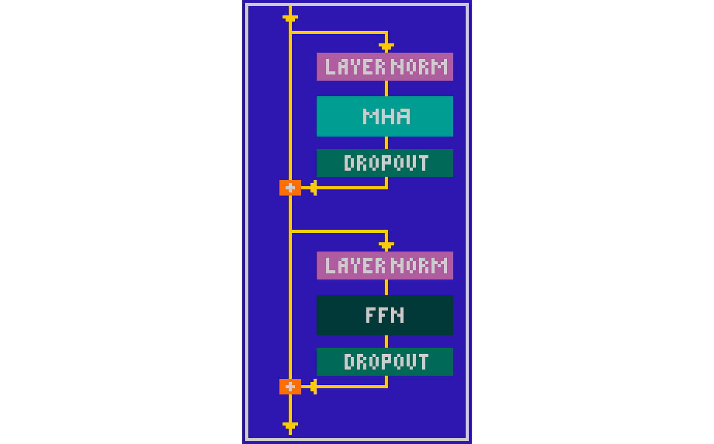
Transformer block

Almost every expensive op in a transformer is a matrix multiplication. Tokens get multiplied by Wq, Wk, Wv, Wo for attention and by Win and Wout in the MLP.

Attention

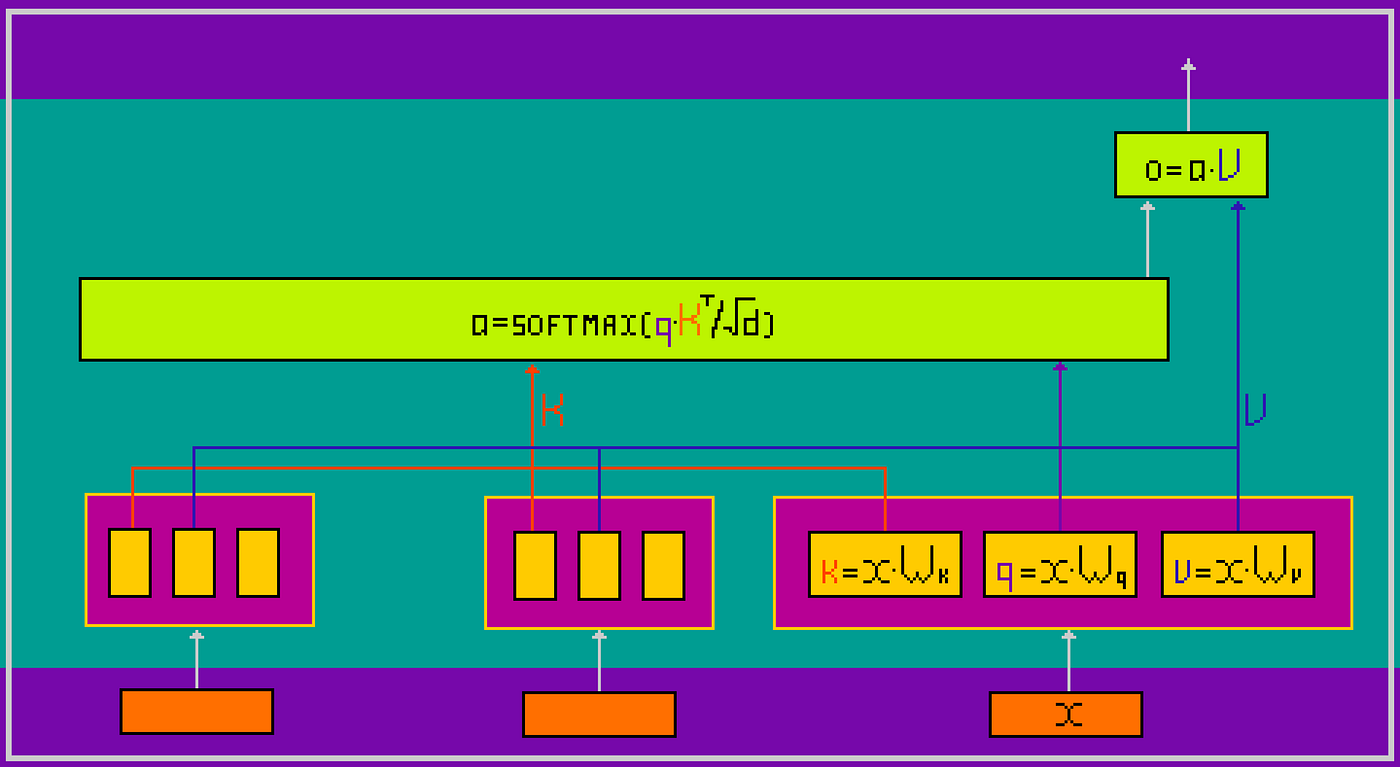
One-Head attention

MLP block

Here’s the MLP inside a transformer block: a layer norm, an “up” projection Win that expands the hidden size from d to f, a nonlinearity (GELU, SwiGLU, whatever you fancy), a “down” projection Wout that brings it back, and a dropout.

X = LayerNorm(X) X = X Win X = Nonlinearity(X) X = X Wout X = Dropout(X)

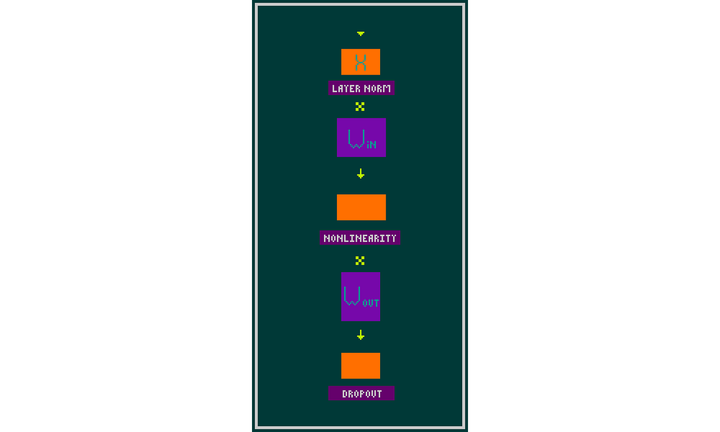
MLP block

If you can split a matmul across devices, you can split the model.

Matrix Multiplication

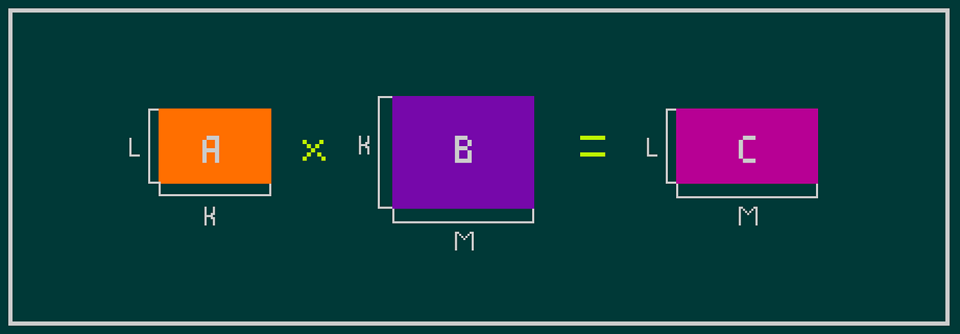
Two matrices in, A and B ( L x K and K x M), one matrix out, C (L × M). Each entry C[i, j] is the dot product of row i of A with column j of B:

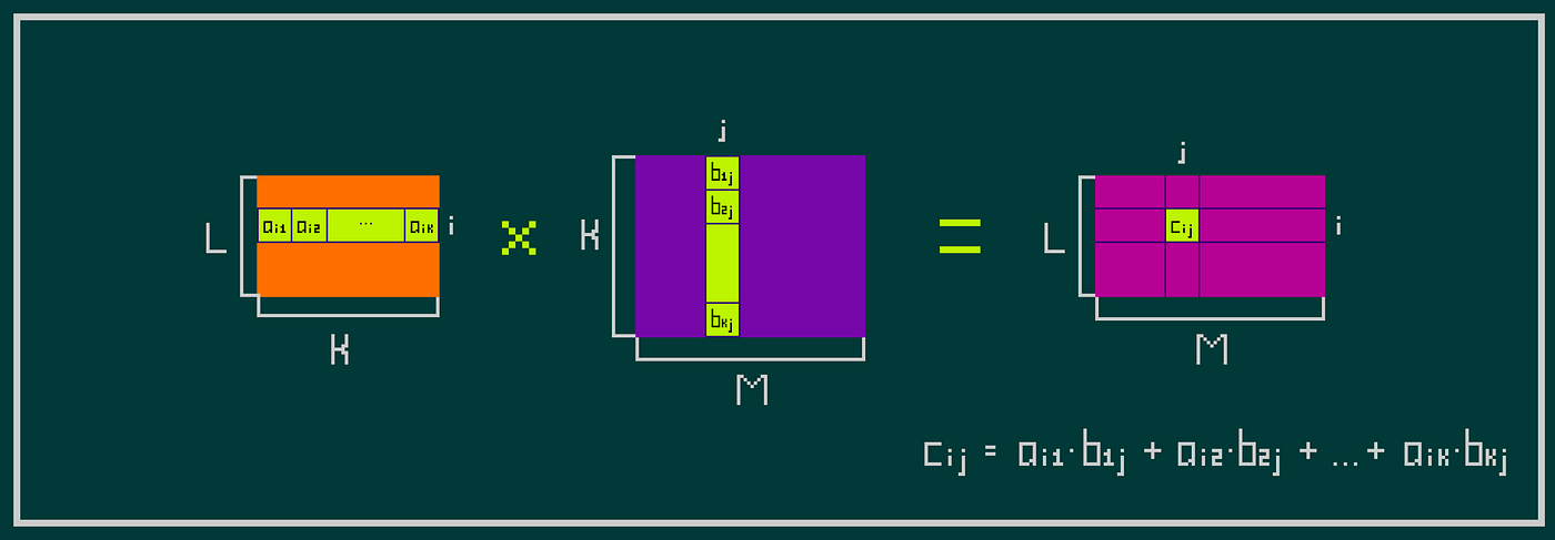
Two things to notice, because they are the two ways tensor parallelism shards a matrix:

1. Different output columns of C are completely independent of each other from the point of view of matrix B. Computing column j only touches column j of B — never column j+1. So you can hand each device a different slice of B’s columns and let them work in parallel without saying a word to each other.
2. The dot product itself — that big sum over k — is associative. You can split the inner index k into chunks, compute each chunk on a different device, and add the partial sums at the end. The result is identical.

Those two observations give us the two flavors of tensor parallelism.

Tensor parallelism, take one: split the output dimension

The first option is column parallelism. We slice the right-hand matrix B along its M dimension into N pieces of width M/N, send one slice to each device, and replicate A. Every device computes its own narrow slab of the output.

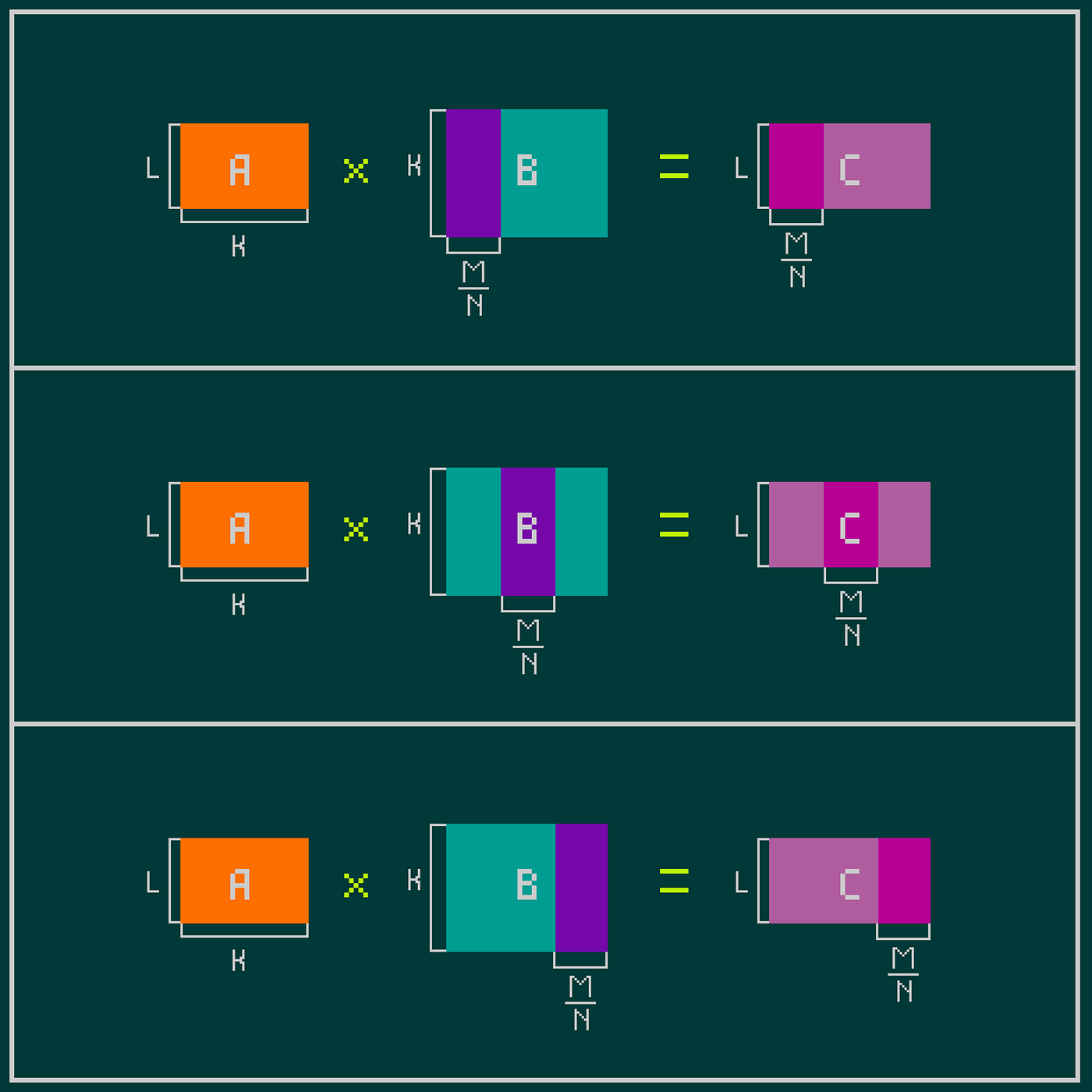
Matrix multiplication with column parallelism

No communication is needed during the matmul itself. Each device just does its own smaller matmul: [L × K] × [K × M/N] = [L × M/N], and it takes 2LKM/N FLOPs. If anyone downstream actually needs the full L × M matrix, you’ll need an all-gather to stitch the slabs back together. About data exchange processes you can read in Collective operations used in LLM training.

Tensor parallelism, take two: split the inner dimension

The second option is row parallelism. Now we split the K dimension itself. Here two matrices in, A and B (L x M and M x K), one matrix out, C (L × K). We give each device a chunk of A’s columns and the matching chunk of B’s rows, then add up the partial results.

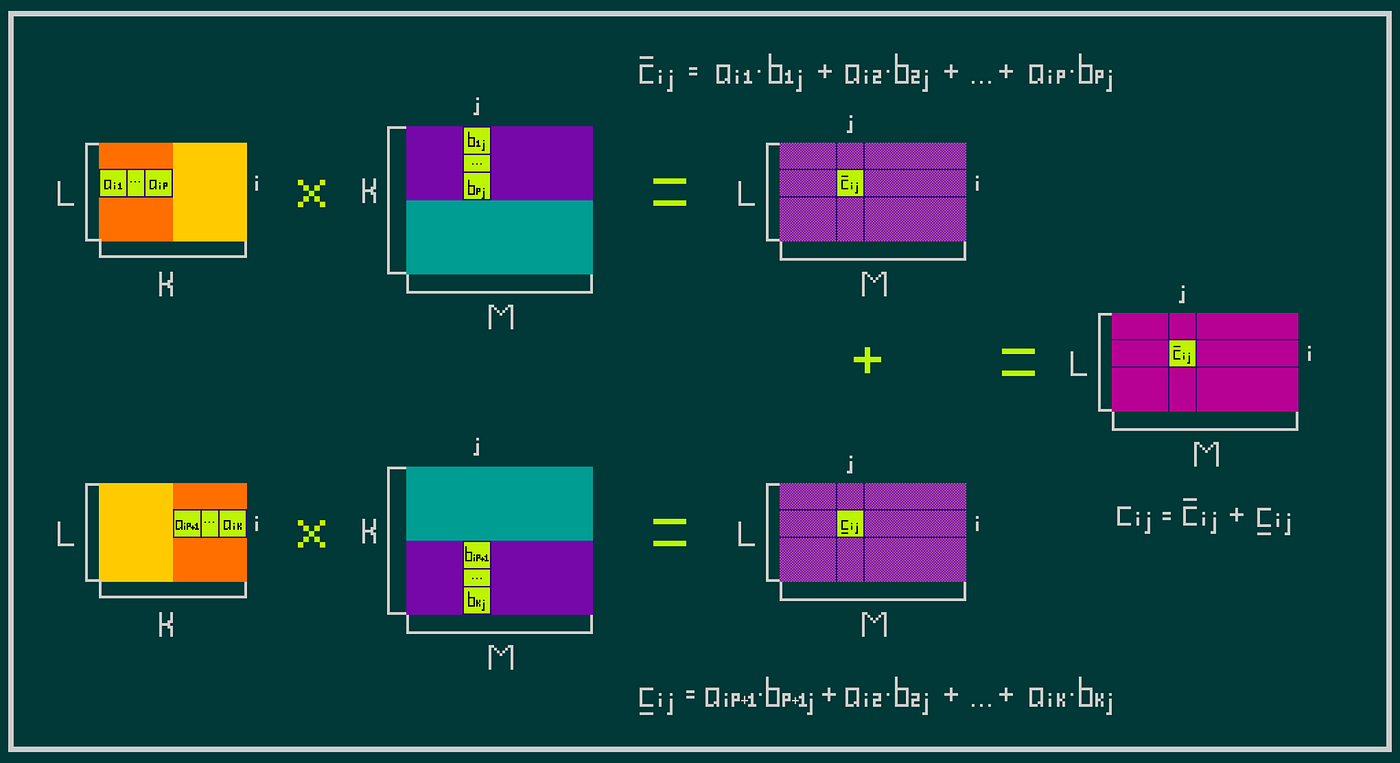
The same idea can be done with dividing matrix B by N row chunks. Each device computes a full-shape L × K partial output from its slice of the inner dimension (it takes 2LKM/N FLOPs), and we sum them across devices to get the final answer.

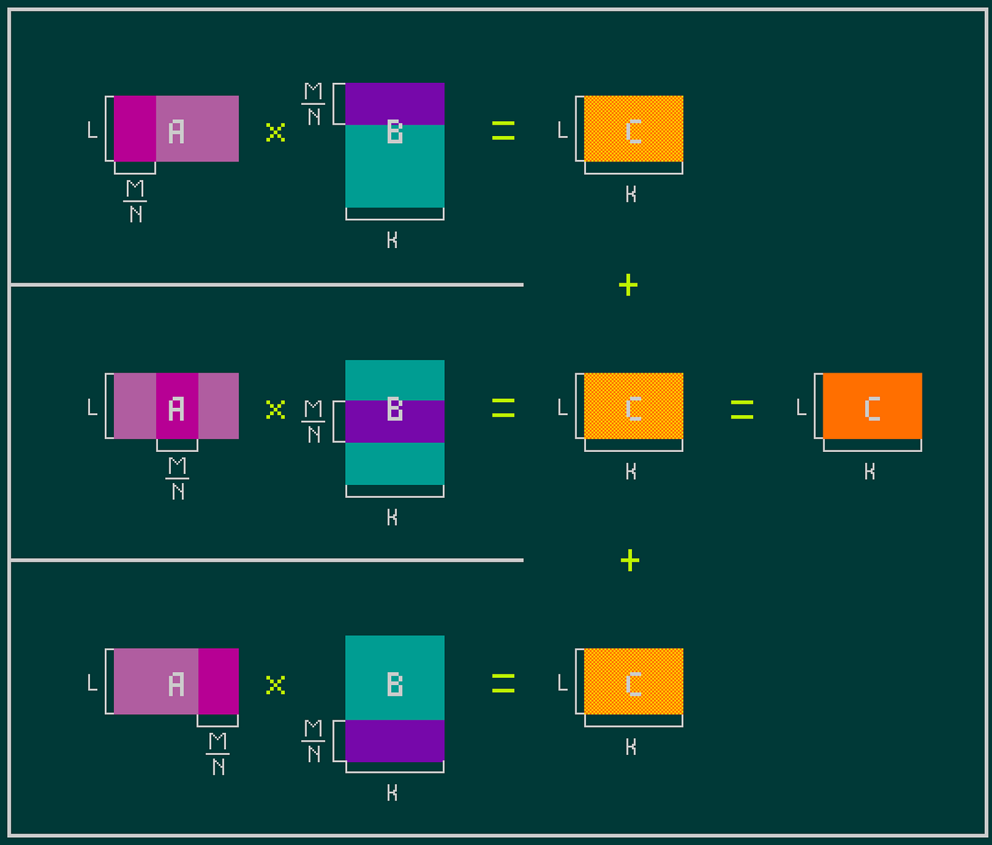
Adding row parallelism

Row parallelism requires communication at the end: every device has only a partial sum, and the partials have to be combined across the group. There are different collective operations that can do this — we meet two of them later — and the choice of collective is exactly what distinguishes vanilla tensor parallelism from the tensor + sequence parallelism setup the diagrams in this post show.

Only Tensor parallelism

The recipe for the MLP block is:

• Win is column-parallel. Each device holds [d, f/N] and computes X · Win, getting an output of shape [batch, seq, f/N]. No comms needed yet — X is replicated across devices.
• The nonlinearity is applied locally. GELU is element-wise; sharding the hidden dimension doesn’t change anything.
• Wout is row-parallel. Each device holds [f/N, d]. It takes its local [batch, seq, f/N] activations and produces a partial [batch, seq, d]. Add an all-reduce across devices and you have the full output.

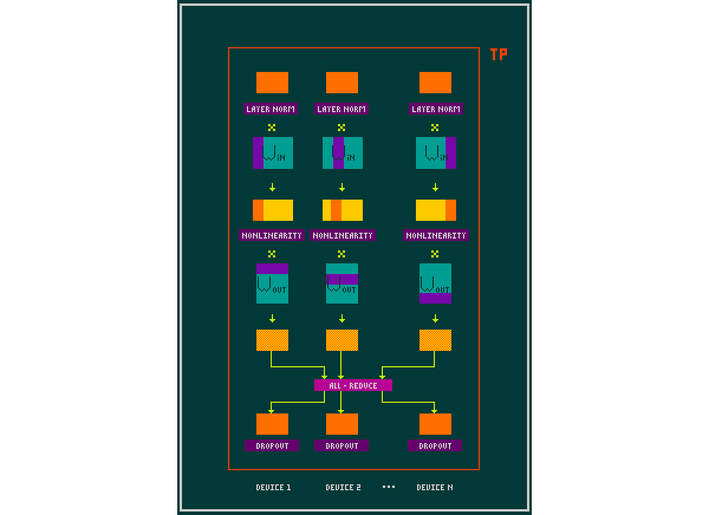
Two matmuls, one all-reduce. No communication at all between them, and the giant f-dimensional intermediate activation is sharded N ways automatically.

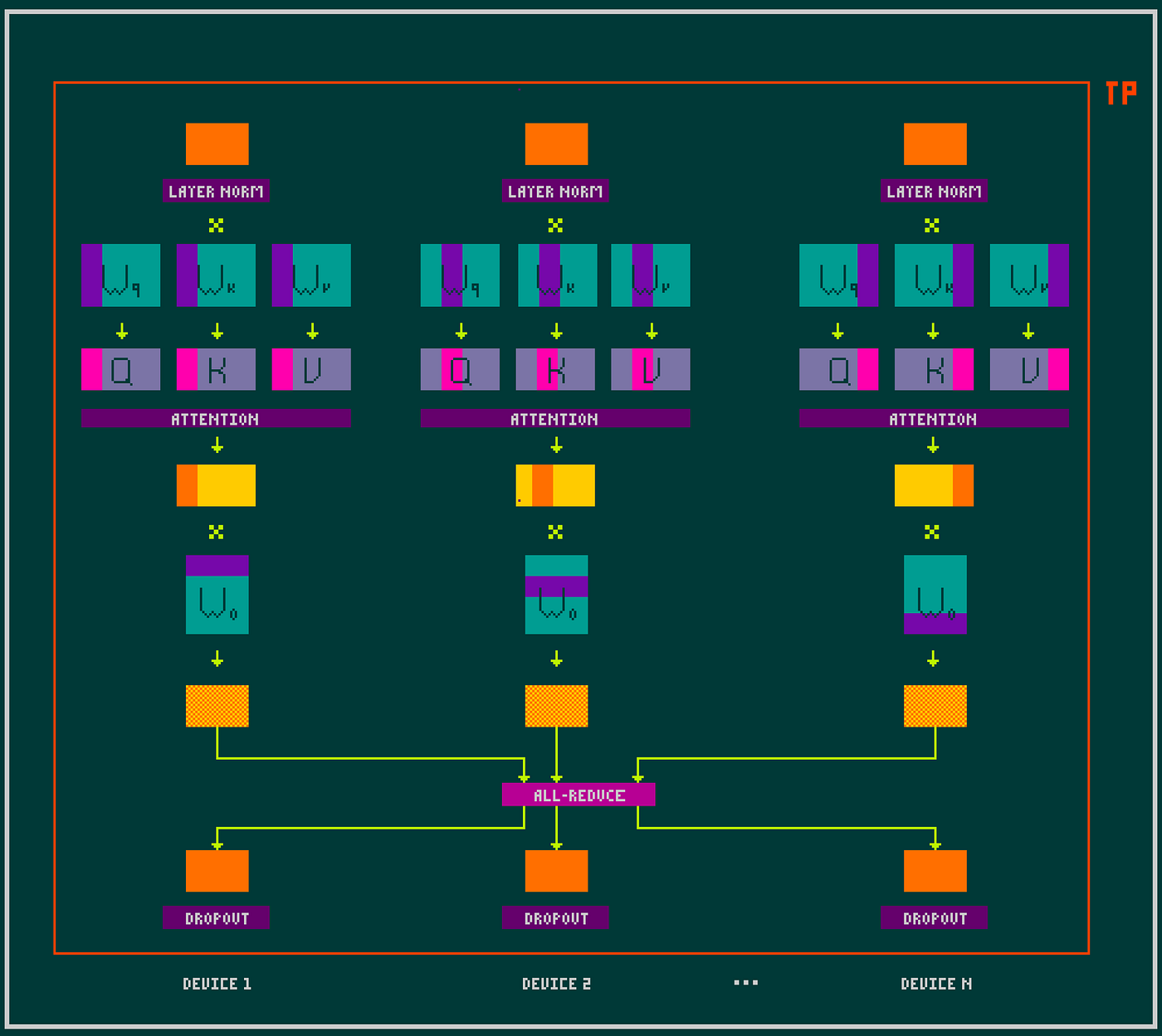
The same trick works for self-attention with Wq, Wk, Wv column-parallel — TP shards the head dimension, Wo row-parallel, one all-reduce per block.

Add Sequence parallelism

Look at the MLP block again. Tensor parallelism sharded the hidden dimension across devices, but a few operations were left replicated on every device:

• LayerNorm, before Win
• Dropout, after Wout
• The residual connection that wraps the block

These are all elementwise. They have nothing to do with the hidden dimension being whole — they just need each token’s vector to be intact at that position. So the sequence dimension is fair game.

The sequence-parallelism observation (Korthikanti et al., 2022) is: split these elementwise operations along the sequence dimension. Device i only sees its sequence-length/N-token chunk during LayerNorm and Dropout. Activation memory for those layers drops by N× with no extra compute.

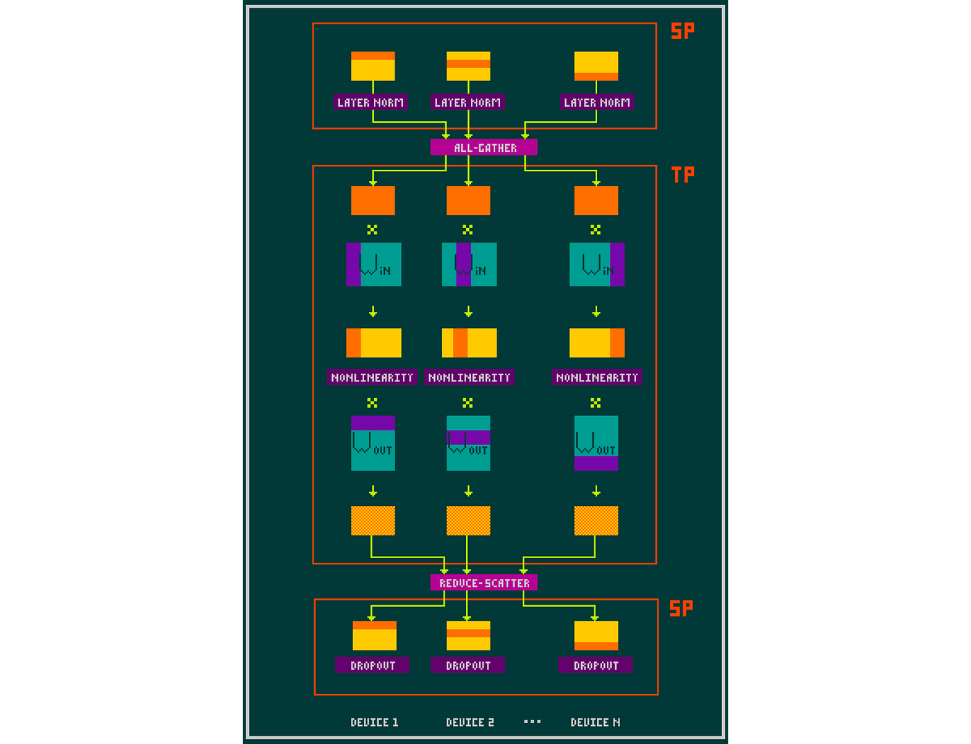
Reading that diagram top to bottom: each device starts with its sequence shard. Apply LayerNorm locally. All-gather to get the full sequence. Run the column-parallel Win, the non-linearity, and the row-parallel Wout exactly as in plain TP. Reduce-scatter the output back to a sharded representation. Apply Dropout locally. Done. The whole transformer block stays in this SP → TP → SP pattern, with collectives only at the boundaries.

And here is the magic: an all-gather plus a reduce-scatter is exactly the same total volume as the all-reduce we already had to do for vanilla TP. Same wire cost, less activation memory.

And the same trick also works for self-attention.

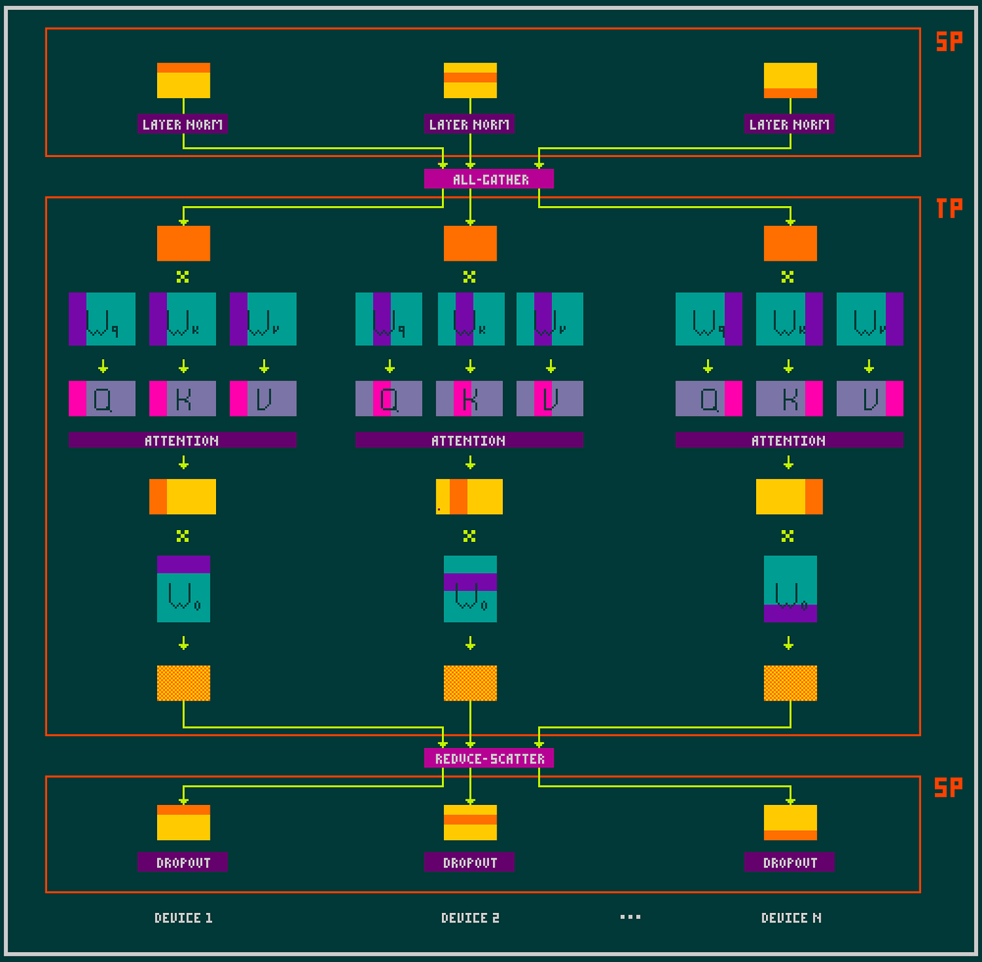
In production training stacks, TP+SP is the default: you almost always want it together.

Wrapping up

One transformer block, sharded across many devices. Tensor parallelism splits the weights along the hidden dimension — column-parallel up-projection, row-parallel down-projection — so per-device weight memory and the wide intermediate activation both shrink dramatically. Sequence parallelism splits the elementwise bookends (LayerNorm, Dropout, residual) along the sequence dimension; the all-reduce that closed pure tensor parallelism becomes an all-gather followed by a reduce-scatter, for the same wire cost and a matching shrink in replicated activation memory.

Together they form the default building block of modern training and inference stacks.

Links and references

• **Visualization of data parallelism** post
• **Collective operations used in LLM training** post
• **Megatron-LM: Training Multi-Billion Parameter Language Models Using Model Parallelism** — Shoeybi et al., 2019. The original tensor-parallel MLP and attention partitioning
• **Reducing Activation Recomputation in Large Transformer Models** — Korthikanti et al., 2022. Introduces the SP + TP combination diagrammed above
• **The Ultra-Scale Playbook (Hugging Face)** — a very readable end-to-end overview of large-scale training