AI/ML in Statistical Compilation, Part 3: Big Data, Non-Probability Samples, and the Last Mile

Why large datasets still need a statistical anchor

Figure 1: A statistical compilation process with AI/ML inside the process

The hardest problem comes last.

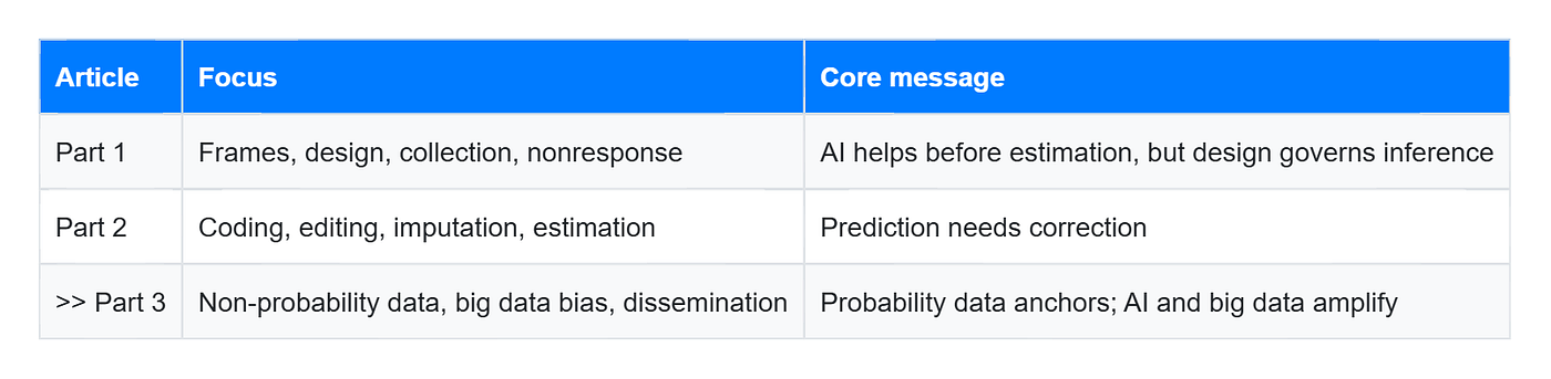
Table 1: Series map of the article

The section lettering continues from Part 1 and Part 2, where Sections A–D in Part 1 covered frames, design, collection, and nonresponse; and Sections E–F in Part 2 covered editing/coding, imputation and estimation.

Note: This article is a practitioner-oriented synthesis rather than an exhaustive methods review. The examples are illustrative, and I welcome corrections, additions, and comments from survey statisticians, official-statistics practitioners, and data scientists.

What happens when the data are large, cheap, timely, and rich — but not sampled probabilistically?

This is the world of opt-in panels, app data, platform records, transaction streams, loyalty databases, web surveys, scraped systems, and commercial data.

These sources are tempting because they are enormous. But survey inference asks a harsher question:

Who had a chance to appear in the data, and what was that chance?

In a probability sample, each unit has a known inclusion probability:

In a non-probability source, πᵢ​ is unknown. For some groups, it may be effectively zero.

That is the non-probability frontier.

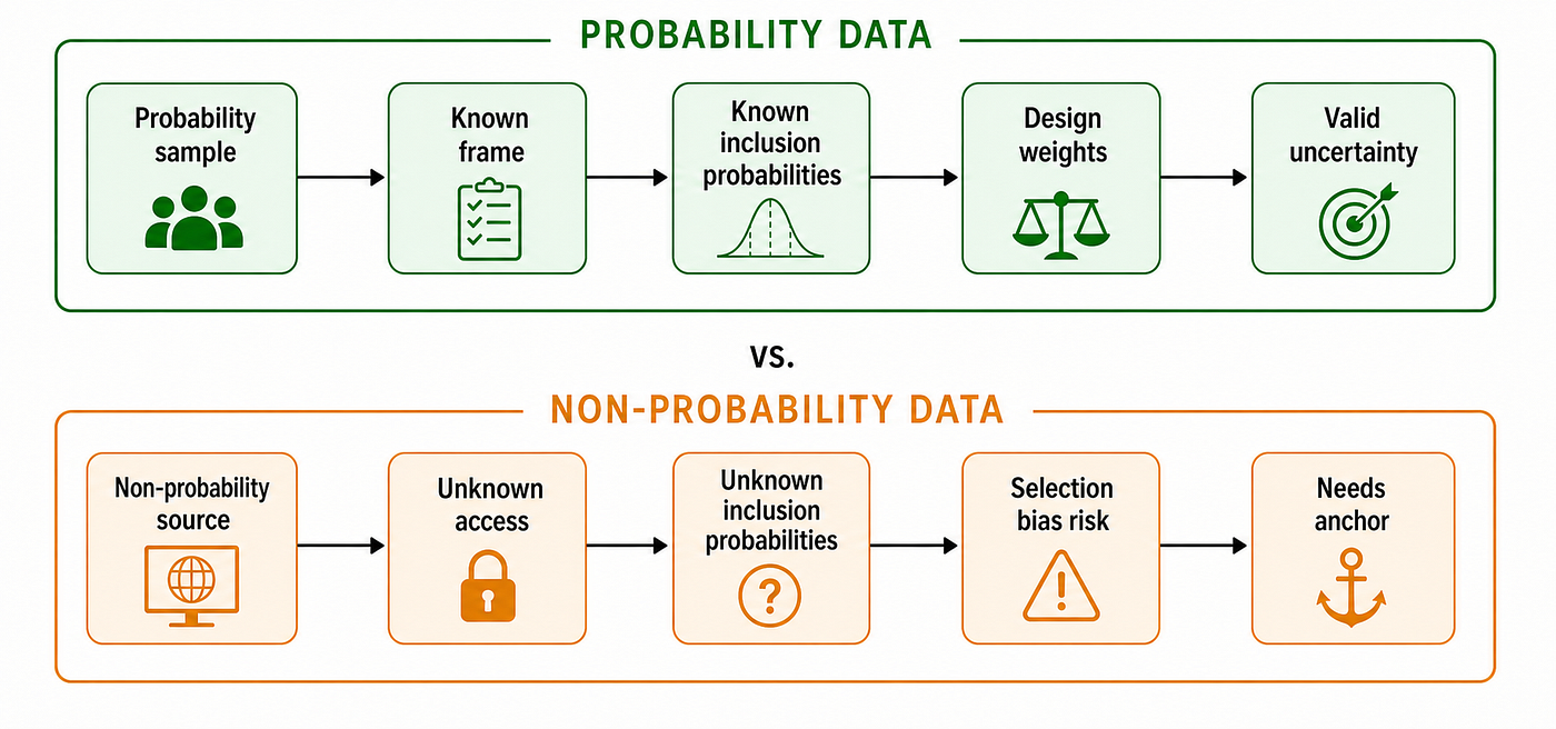
Figure 2: Probability data vs non-probability data

The Big Data Paradox

Xiao-Li Meng’s Big Data Paradox gives the sharpest warning against naive reliance on data volume.

For a dataset of size n from a population of size N, let f = n/N, and let ρY,S​ be the correlation between the outcome Y and inclusion in the dataset S. A simplified form of the error is:

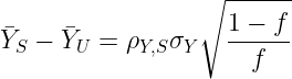
The dangerous term is not simply sample size. It is the data-defect correlation, ρY,S​. Professor Meng shows that even tiny selection-outcome correlations can sharply reduce the effective information in a massive dataset.

An approximate effective sample size expression is:

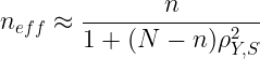
For example, if n = 100,000,000, N = 330,000,000, and ρY,S = 0.033, then the effective sample size is only about 400.

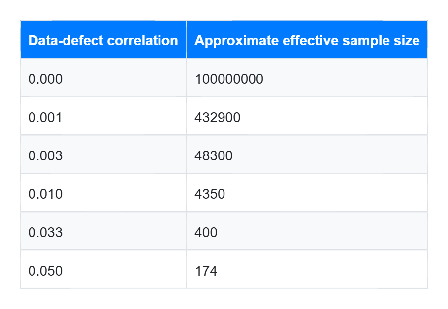
Table 2: Approximate effective sample size for n=100,000,000 and N=330,000,000 under different data-defect correlations

That is the paradox.

More data reduces random noise. It does not automatically reduce selection bias.

A biased dataset does not become unbiased by getting larger. It becomes more confidently wrong.

In practice, ρY,S​ is usually unknown. That is precisely why probability anchors, benchmark comparisons, and sensitivity analysis matter.

G. Anchoring non-probability samples with probability data

The goal is not to pretend a non-probability sample is random. The goal is to use a probability sample, benchmark data, or high-quality auxiliary information to adjust, model, or validate the larger non-probability source.

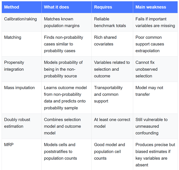
Table 3: Methods for integrating probability and non-probability data

Method 1: calibration, raking and matching

Calibration and raking adjust sample weights so that weighted totals match known population margins. Matching selects non-probability cases that resemble cases from a probability reference sample.

Pew Research Center has tested raking, matching, propensity weighting, and combinations of these methods for online opt-in samples. Its work notes that random forests can be used to construct similarity measures or propensity adjustments that capture relationships missed by simpler raking methods.

The central lesson from Pew’s work is not that complex methods always win. It is that adjustment works only on the variables it can see, and the right auxiliary variables matter enormously.

Method 2: propensity-score integration

A common workflow is:

1. Stack the probability sample and non-probability sample.
2. Create an indicator Sᵢ = 1 if case i came from the non-probability sample.
3. Fit a model e_{hat}ᵢ = P(Sᵢ = 1 ∣ Xᵢ) using logistic regression, random forest, XGBoost or another classifier.
4. Weight or match non-probability cases using the estimated selection or source-inclusion propensity;
5. Calibrate to population totals;
6. Trim extreme weights;
7. Publish sensitivity analysis.

Note: The probability sample should be represented with its survey weights or benchmark population totals; otherwise, the model estimates membership in the stacked file rather than participation relative to the target population.

An inverse-odds adjustment may use weights proportional to:

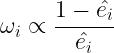
The intuition is simple: units overrepresented in the non-probability source receive less weight, while units underrepresented receive more.

But this works only if Xᵢ​ contains the variables that drive both selection and the outcome. It also requires overlap: the non-probability source must contain enough cases comparable to the target population. If some population groups are absent, the weights become unstable or the model extrapolates.

Very small e_{hat}ᵢ can create extreme weights, so trimming, diagnostics, and sensitivity analysis are essential.

A published COVID-19 application in Spain compared logistic regression with XGBoost for propensity-score estimation when integrating probability and non-probability survey data using calibration and propensity-score integration. In the simulation study, the calibration-plus-propensity-score approach reduced self-selection bias and root mean square relative error, with boosting-based propensity models generally outperforming comparable logistic-regression models. In the empirical application, the authors treated the calibration-plus-XGBoost estimator as more reliable than direct calibration of the merged sample alone, while noting that nonresponse in the probability sample still required careful attention.

Method 3: mass imputation

Mass imputation flips the usual roles of the two samples.

Suppose the non-probability sample s_NP​ is large and contains the outcome y, while the probability sample s_P is smaller and contains valid design weights dᵢ = 1/πᵢ​, but lacks y. Both sources contain shared covariates x.

Fit the outcome model on the non-probability sample:

Then impute the outcome onto the probability sample:

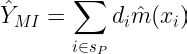
The probability sample carries the population structure. The non-probability sample supplies the outcome relationship.

Note: This is worth contrasting with the model-assisted estimation in Part 2. In model-assisted estimation, the outcome model was fitted on the probability sample and corrected by its own residuals. In mass imputation, the outcome model is fitted on the non-probability sample and transported onto the probability sample. The direction of borrowing has reversed — and with it, the assumptions.

This approach has been developed in the survey-sampling literature as a way to combine probability and non-probability samples through mass imputation.

Mass imputation depends on two assumptions:

1. Transportability: E(y ∣ x) is the same in the non-probability source and the target population.
2. Common support: the non-probability source and the probability sample should have sufficient overlap in the distribution of key covariates, so that cases in the non-probability source can be reasonably compared with similar cases in the probability sample.

A further practical requirement is measurement equivalence: the outcome y must mean the same thing in the non-probability source as in the target population or probability reference.

If a group is missing from the non-probability source, the model is extrapolating, not imputing.

Variance is also critical. A naive variance formula treats m_{hat} as known, but it is estimated. Schematically, valid uncertainty must reflect both the probability sample and the fitted prediction model:

Ignoring the second term produces confidence intervals that are too narrow.

Method 4: doubly robust estimation

Doubly robust estimators combine a participation model and an outcome model. Chen, Li, and Wu developed doubly robust inference methods for non-probability survey samples and applied them to a Pew Research Center non-probability sample with auxiliary information from the Behavioral Risk Factor Surveillance System and the Current Population Survey.

The appeal is familiar: under suitable conditions, including adequate common support and relevant auxiliary variables, consistency may hold if either the participation model or the outcome model is correctly specified.

But the warning is also familiar:

Double robustness is not magic. It protects against some model misspecification, not against missing variables, absent population groups, or a non-comparable measurement process.

If selection depends on variables absent from both models, the method cannot fully repair the bias.

Note: This is the same doubly robust logic used in Part 2, but the interpretation changes. Where Part 2 used a response propensity for nonresponse among sampled units, here the same weight uses a participation propensity (for opt-in panels) or source-inclusion propensity (for administrative or platform data) into the non-probability source.

Method 5: MRP for Non-Probability Samples

Multilevel regression with poststratification (MRP) can also help with non-probability data.

A large opt-in panel may be badly imbalanced overall, but still contain enough cases to estimate relationships across demographic and geographic cells. A multilevel model can smooth sparse cells, and poststratification can re-aggregate predictions to real population counts.

MRP works by:

1. modelling the outcome using individual and area-level predictors;
2. predicting outcomes for poststratification cells;
3. aggregating predictions using known population cell counts.

The poststratification step is:

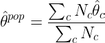
where θ_{hat}c​ is the fitted model outcome for cell c, and Nc is the known population count for cell c.

Note: The mechanics are identical to Part 2. The difference is that the input is now a self-selected panel rather than a probability sample.

An MRP example applied to a non-probability panel: YouGov’s MRP and the 2017 UK general election

YouGov’s 2017 UK general-election model used MRP to produce constituency-level estimates and correctly indicated that the country was heading towards a hung parliament. The London School of Economics and Political Science also described the model as one of the few to correctly predict a hung parliament when many conventional forecasts expected a Conservative majority.

The model used a very large volume of online panel data — around 7,000 panellist interviews per day and about 50,000 per week. YouGov modelled voting intention as a function of constituency, voter demographics, past voting behaviour and other profile variables, then poststratified those predictions to estimated constituency-level voter compositions using sources such as the Office for National Statistics in the UK, the British Election Study and past election results.

This was not a conventional probability sample with known inclusion probabilities. YouGov itself contrasted the MRP model’s large weekly data stream with its more traditional carefully selected polling samples.

The methodological lesson is not that large panels remove sampling problems. The lesson is that large non-probability data can be useful when they are disciplined by strong auxiliary information, explicit modelling, poststratification and uncertainty reporting.

This is why MRP became so influential in modern polling. It can convert noisy individual responses into stable estimates for states, districts, constituencies, or demographic subgroups.

The panel supplied scale. The poststratification frame supplied structure. Neither supplied known inclusion probabilities.

But the two load-bearing assumptions from Part 2 now do heavier work:

MRP corrects imbalance only on variables included in the model and poststratification frame. The poststratification cell counts must also be reliable and aligned with the target population.

If opt-in panellists differ from non-panellists in unmeasured ways, MRP may produce precise but biased estimates. With a probability sample as in Part 2, there is at least a documented inclusion mechanism and design-based reference point; with a non-probability opt-in panel, there is no such backstop.

Hybrid Inference: Anchor Plus Amplifier

The answer is not to discard non-probability data. That would waste valuable information.

The answer is also not to blindly trust it. That would be reckless.

The future is hybrid inference:

The probability source provides the anchor. The non-probability source provides the scale.

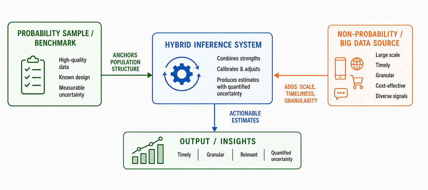
Figure 3: The non-probability source supplies scale. The probability source supplies credibility

A practical hybrid-inference workflow is to:

1. define the target population, units, reference period and domains of interest;
2. specify the estimand, including the outcome variable and target population quantity to be estimated;
3. obtain a probability-sample anchor, or at least strong external population benchmarks;
4. harmonise definitions, measurement, timing and covariates across probability and non-probability sources;
5. assess coverage gaps, overlap and common support between the data sources and the target population;
6. model key data-generating mechanisms, including participation in the non-probability source, nonresponse in the probability sample, and the outcome process where needed;
7. use calibration, propensity weighting, poststratification, mass imputation or related methods to align the combined data with the target population;
8. validate estimates against independent or held-out benchmark quantities that were not used directly in fitting or calibration;
9. assess sensitivity to unobserved selection, model misspecification, coverage error and benchmark error;
10. publish estimates with uncertainty measures that reflect sampling error, weighting, imputation, calibration and model uncertainty.

This is where AI/ML is genuinely useful. It can improve matching, estimate participation propensities, model nonlinear outcome relationships, support MRP, and power mass imputation.

But credibility still comes from the anchor.

Non-probability data can amplify statistical production, but only a probability sample, benchmark, or trusted frame can anchor inference.

H. Dissemination and User Support: Conversational AI

Every section so far has followed statistics from frame to estimate. But the compilation process does not end when a number is published.

It ends when a user finds that number, understands it, and uses it correctly.

This last mile is exactly where large language models and chatbots are arriving fastest. It also carries a distinctive risk: when a statistical office attaches its name to an answer, a confident wrong answer damages trust more than no answer at all.

A statistical office’s numbers are only as valuable as the public’s ability to find and understand them. Dissemination is not an afterthought to statistical compilation — it is its final stage.

Example H1: Statistics Singapore’s SANDRA

The Singapore Department of Statistics (DOS) maintains the SingStat Table Builder, which provides access to roughly 2,400 customisable datasets from about 70 public-sector agencies and around 150,000 data series across economic and socio-demographic domains.

That comprehensiveness is a strength, but also a discoverability problem. A user asking “How many households own cars?” or “What has happened to life expectancy?” may not know the correct table title, subject category, statistical concept, or metadata wording.

SANDRA — the Statistics ANd Data Retrieval A.I. assistant — addresses that problem. SANDRA is an AI chatbot using natural language and large language models to assist users with data enquiries using data in SingStat Table Builder.

The strategic logic is simple:

National statistical offices invest enormous effort producing accurate figures. But much of that value is stranded if users cannot locate the right series.

SANDRA converts a browse-the-taxonomy experience into an ask-a-question experience. Users can ask questions in ordinary language and receive relevant datasets without knowing exact table names or technical terminology. Staff resources can also be freed for complex or high-value questions.

The development of this AI chatbot can be divided into four stages:

1. Discovery through search-log analysis and stakeholder interviews;
2. Design around user intent;
3. Detailing through metadata modelling and vector embeddings for the time-series datasets; and
4. Development and deployment of the interface, retrieval logic, and secure cloud environment.

The key design principle is that SANDRA should retrieve from a trusted, curated corpus rather than generate official statistics from a language model’s parameters. For official-statistics assistants, the safeguards are as important as the interface: answers should be source-linked, metadata-aware, time-stamped, and able to say “no result found” when retrieval confidence is low.

Formally, given a user query q, the system retrieves the datasets whose embeddings are most semantically similar:

where ϕ(q) is the embedding of the query, ϕ(d) is the embedding of dataset metadata, and C is the curated official-statistics corpus.

The assistant can then present the retrieved series as a chart or table, with metadata, related datasets, and links back to the official source.

Retrieval, not fabrication, is the whole design.

In modern AI terminology, this is a retrieval-augmented design: the language model supplies the conversational layer, while the official data source supplies the authority.

This is the difference between a grounded official-statistics assistant and a generic chatbot.

The language model supplies fluency. The retrieval system supplies authority.

Final Conclusion: AI/ML Strengthens the System, Design Makes It Trustworthy

Trace the statistical compilation pipeline from beginning to end:

1. frame construction;
2. sampling design;
3. data collection;
4. nonresponse adjustment;
5. coding and editing;
6. imputation;
7. estimation;
8. non-probability integration (where applicable);
9. dissemination and user support.

The same pattern appears at every stage.

AI/ML is powerful when it helps statisticians do the work better: build frames, classify text, detect anomalies, target fieldwork, model missingness, improve precision, retrieve official data, and support users.

But AI/ML is dangerous when it hides the inferential structure. Probability selection, coverage assessment, known inclusion probabilities, transparent edits, honest weighting, credible uncertainty, and grounded dissemination remain the load-bearing structure of official statistics.

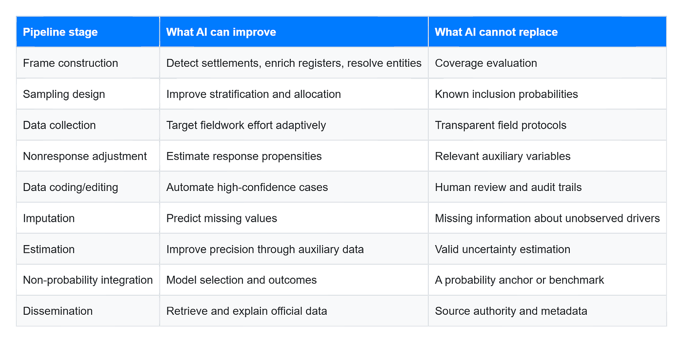
Table 4: What AI/ML can improve and what AI/ML cannot replace in a statistical production process

There is also a governance layer. AI/ML-assisted official statistics require documented data provenance, privacy protection, reproducible pipelines, model monitoring, access controls, audit trails, and clear public communication. A model that improves accuracy but cannot be explained, audited, or reproduced may still be unsuitable for official statistical compilation.

The best architecture is not AI/ML instead of statistical design.

It is:

AI/ML inside statistical design.

That is the durable lesson.

AI/ML can strengthen statistical compilation — but it does not replace statistical design.

👉 Haven’t read **part 1 yet?**

👉 Read the Chinese version **here**

References

1. Chen, Y., Li, P., & Wu, C. (2020). Doubly robust inference with nonprobability survey samples. Journal of the American Statistical Association, 115(532), 2011–2021.
2. Kim, J. K., Park, S., Chen, Y., & Wu, C. (2021). Combining non-probability and probability survey samples through mass imputation. Journal of the Royal Statistical Society Series A: Statistics in Society, 184(3), 941–963.
3. London School of Economics and Political Science. (2017). LSE pollsters win the day.
4. Meng, X.-L. (2018). Statistical paradises and paradoxes in big data (I): Law of large populations, big data paradox, and the 2016 US presidential election. The Annals of Applied Statistics, 12(2), 685–726.
5. Mercer, A., Lau, A., & Kennedy, C. (2018). How different weighting methods work. Pew Research Center.
6. Mercer, A., & Lau, A. (2023). Comparing two types of online survey samples. Pew Research Center.
7. PebbleRoad. (2025). How conversational AI unlocked Singapore’s national data asset.
8. Rivers, D. (2017). How the YouGov model for the 2017 General Election works. YouGov.
9. Rueda, M. M., Pasadas‐del‐Amo, S., Cobo Rodríguez, B., Castro‐Martín, L., & Ferri‐García, R. (2022). Enhancing estimation methods for integrating probability and nonprobability survey samples with machine‐learning techniques. An application to a Survey on the impact of the COVID‐19 pandemic in Spain. Biometrical Journal, 64(8), 1423–1441.
10. Shakespeare, S. (2017). Two methods, one commitment: YouGov’s polling and model at the 2017 election. YouGov.
11. Shakespeare, S. (2017). How we correctly called a hung parliament. YouGov.
12. Singapore Department of Statistics. (2026). SingStat Table Builder.
13. Singapore Department of Statistics. (2026). DOS AI and Generative AI Playbook.
14. Singapore Department of Statistics. (2026). About SANDRA.
15. YouGov. (n.d.). Methodology.