RECAP, Explained: How π*₀.₆ Turns Advantage Conditioning Into a VLA That Learns From Experience

A technical walk through the method behind Physical Intelligence’s π*₀.₆ — the preliminaries, the distributional critic, and the advantage-conditioning objective — with the key equations explained plainly.

Vision-language-action (VLA) models are usually trained by imitation, which caps them at the quality of their demonstrations and gives them no way to learn from their own failures. RECAP (RL with Experience and Corrections via Advantage-conditioned Policies) is Physical Intelligence’s recipe for breaking that ceiling: pre-train a generalist VLA with offline RL, then specialize it on-robot using autonomous rollouts and human corrections. The resulting model, π*₀.₆, folds laundry in real homes, assembles boxes, and makes espresso — more than doubling throughput and roughly halving failure rate on the hardest tasks.

This post focuses on how the method works, building from the RL preliminaries up to the actual training objective.

1. The RL setup, precisely

A policy π(aₜ | oₜ) is a distribution over actions aₜ given an observation oₜ. Rolling it out produces a trajectory:

an alternating sequence of observations and actions. Note the asymmetry: T+1 observations, T actions — the episode begins and ends on an observation.

The probability of a trajectory under the policy is the trajectory distribution, induced jointly by the policy and the environment’s dynamics p(oₜ₊₁ | oₜ, aₜ):

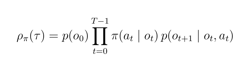
Two sources of randomness interleave here — the policy (which you control) and the dynamics (which you don’t). The clean product form holds only under the Markov assumption that oₜ is a valid state; the paper flags this as a standard robotic-RL simplification, not literally true for a robot with occlusions and momentum.

A per-step reward r(oₜ, aₜ) = rₜ accumulates into the return R(τ) = Σₜ rₜ. The paper uses no discount factor (γ = 1) — its episodes are finite-horizon, so the sum converges without one, and it doesn’t want to artificially prefer earlier reward. The objective is expected return:

The thing to notice: π appears twice — inside R(τ) (better actions earn more reward) and inside ρπ (the policy also changes which trajectories occur). Optimizing π reshapes the very distribution you’re averaging over. That’s what makes RL harder than supervised learning.

The value function is expected reward-to-go from a state, Vπ(oₜ) = E[Σ{t′≥t} r{t′}], and the advantage measures how much a specific action beats that baseline, as an n-step estimate:

Read it as (estimated return if you take aₜ) − (baseline value of being at oₜ). The N-step truncation — trust N real rewards, then bootstrap with V — is a bias/variance dial between pure Monte-Carlo (N→∞, unbiased, high variance) and one-step TD (N=1, low variance, biased).

2. Regularized RL: the theoretical hook

Pure reward maximization on a fixed dataset is dangerous: train many gradient steps and the policy drifts into regions the data can’t support, exploiting estimation errors. The fix is regularization — improve reward while staying close to a reference policy π_ref (typically the behavior policy that collected the data):

β controls leash tightness. For KL divergence there’s the classic closed form:

i.e. “the reference policy, reweighted toward high-advantage actions” (the basis of AWR/MARWIL/MPO).

RECAP uses a related, less common form. Define improvement probability p(I | A) = g(A)/∫g(A′)da′ for any monotonically increasing g, and set:

This π̂ carries a provable improvement guarantee: J(π̂) ≥ J(π_ref). That guarantee is the bedrock that lets RECAP loop safely. Finally, you project this closed form onto a trainable network by minimizing KL(π̂, π_θ).

3. The distributional value function (the critic)

RECAP represents Vπref as a multi-task distributional value function p_φ(V | oₜ, ℓ) over B = 201 discretized bins, conditioned on observation and language command ℓ. It shares the VLA’s architecture but uses a smaller VLM backbone.

Training turns value regression into classification: discretize the empirical return Rₜ(τ) = Σ{t′≥t} r{t′} into bins, then minimize cross-entropy. Why distributional rather than a single regressed number?

• Stability — cross-entropy classification is far more stable to optimize than regression at scale.
• Uncertainty — a histogram can express “I’m unsure” (wide spread) vs. “confident” (sharp peak).
• Multimodality — states that lead to either success or failure get two honest peaks instead of a misleading average.

Concretely, the reward they use is steps-to-success, normalized to (−1, 0) with 0 = completion. So the critic predicts a distribution over time-to-completion — which is exactly why it “detects failures and judges expected time to task completion.”

Critical detail when scoring data: to get a scalar value from the histogram you take its expected value (probability-weighted mean of the bins), not the argmax / tallest bin. Taking the peak would throw away the spread the distributional critic exists to capture. The advantage then follows from the n-step formula — query the critic at oₜ and at o_{t+N}, add the real rewards in between, subtract. The advantage is computed, never read off as a bin.

So the representations compress in stages: distribution (critic output) → scalar (expected value) → advantage (a number) → tag (one bit).

4. Policy extraction via advantage conditioning

The method needs a policy-extraction step that (a) uses diverse off-policy data — demos, interventions, and rollouts from current and past policies; (b) scales to large VLAs, including flow-matching/diffusion action heads with no tractable log-likelihood; and (c) uses both good and bad data. Policy gradients fail (b); weighted regression (AWR/CRR) effectively discards much of the data via filtering. RECAP instead uses advantage conditioning: train on all data with plain supervised learning, but add an input indicating how optimal each action is.

Applying Bayes’ rule to the improvement probability gives an equivalent closed form (most closely related to CFGRL):

For the special case β = 1 this collapses to simply π̂ = π_ref(a | I, o, ℓ). So you can represent the improved policy without ever explicitly modeling p(I | A) — you just need a policy that can produce actions both with and without the conditioning variable I. This is exactly the classifier-free guidance idea.

The conditioning variable is binary, defined by thresholding the advantage:

with a task-dependent threshold ε_ℓ. (The paper prefers tuning this threshold over tuning a test-time guidance weight β, since high CFG weights drive actions to the corners of their support and don’t affect the autoregressive part of the model.)

The policy objective is a classifier-free-guidance-style negative log-likelihood — modeling the action both unconditioned and conditioned on I:

where α trades off the two terms. At inference, you condition on I = True to elicit the improved behavior.

A few implementation notes worth carrying:

• The dataset D_πref is everything — all demonstrations plus all autonomous attempts. So π_ref is a mixture of human behavior and previously deployed policies, and the advantage tag is what sorts good from bad across that mixture. Both critic and policy train on this full pool — the policy needs the labeled-bad rollout actions to give the tag meaning.
• Human corrections are forced to I = True, on the assumption that expert interventions are always good actions — a cheap, high-quality signal injection.
• π*₀.₆’s action head produces both discrete and continuous outputs (continuous via flow matching), so the real objective combines a likelihood for discrete tokens with the flow-matching objective for continuous actions.

5. The full method

RECAP reduces to three subroutines (Algorithm 1), repeated:

1. Collect autonomous rollouts (with optional expert corrective interventions), labeling outcomes.
2. Train the value function (Eq. 1, distributional cross-entropy).
3. Train the policy via advantage conditioning (Eq. 3).

The only thing that changes between stages is the data fed to each subroutine. Pre-training runs steps 2–3 on the full demonstration dataset (tens of thousands of hours across many robots and tasks). Then each task’s specialist runs steps 1–3 with added autonomous data — specialists are fine-tuned from the pre-trained model, while the final generalist is trained from scratch on the union.

Why the design choices line up

Every piece earns its place against the three criteria:

• Diverse off-policy data → handled by training on the full pool with honest good/bad tags rather than filtering.
• Scales to flow-matching VLAs → advantage conditioning needs no tractable log-likelihood ratio; it’s plain conditional supervised learning plus a flow-matching term.
• Uses good and bad data → the binary indicator lets failures train the model as labeled negatives, instead of being discarded.

The result is a self-improvement flywheel with a provable per-iteration improvement guarantee underneath it — which is what lets a VLA keep getting better from real-world deployment rather than plateauing at imitation quality.

Equations and framing follow the π*₀.₆ paper (Physical Intelligence, 2025); see the original for full implementation details, ablations, and experimental results.