Interactive Brain Activation Maps with Anatomical Labeling: a Python alternative to SPM

One function to generate a clickable HTML brain viewer that returns the anatomical region under your cursor, with an interactive cluster table — built on nilearn, no server required.

When presenting PET or fMRI activation results, the typical workflow stops at a glass brain or a set of axial slices. These are publication-ready, but not exploration-ready.

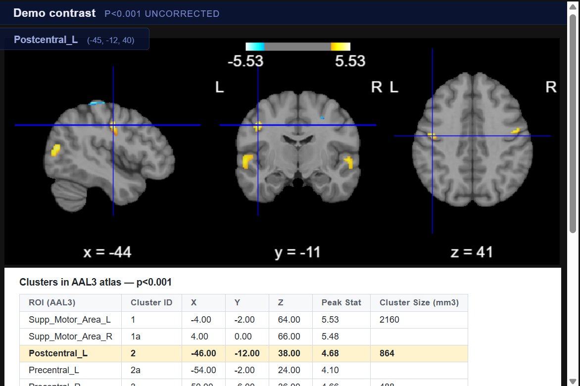
This article describes a self-contained Python function — built on top of nilearn — that generates an interactive HTML brain viewer where:

• clicking any voxel returns its MNI coordinates and its AAL3 anatomical label (but easy to adapt with another one),
• an optional cluster table sits below the viewer, sortable by any column,
• clicking a row in that table moves the crosshair to that cluster’s peak.

The output is a single .html file, fully portable, opening in any browser with no internet connection or local server.

Why nilearn?

nilearn is the de facto standard for neuroimaging visualization in Python. Its view_img function produces a self-contained interactive HTML viewer, rendering three orthogonal planes with a colorbar and threshold control. It handles the full NIfTI pipeline — affine transforms, resampling, masking — transparently.

What nilearn does not do natively: label the anatomical region under the cursor, or link a cluster table to the viewer. The function described here closes both gaps.

Step 1 — Build the AAL3 lookup table

Before generating any viewer, you build a lookup table (LUT) once for the entire session:

from viewer import build_aal_lookup, lut_to_json

lut      = build_aal_lookup(aal_path="AAL3v1_1mm.nii.gz", step_mm=2)
lut_json = lut_to_json(lut)

The function loads the AAL3v1 NIfTI volume (1 mm isotropic, 170 regions), resamples it to step_mm resolution using nearest-neighbor interpolation, and maps every non-zero voxel to its region name. The result is a Python dictionary keyed by "x_y_z" MNI coordinate strings.

**step_mm** controls the resolution of the LUT. The default of 2 mm is a good trade-off: fast to build (~5 s), compact (~3 MB serialized), and accurate enough given typical cluster sizes. Use step_mm=1 for single-voxel precision.

The LUT is serialized to JSON once and reused across all viewers — the intended workflow for a multi-contrast study.

Step 2 — Generate the viewer

Viewer only

from viewer import show_brain_viewer
from nilearn import datasets

bg_img = datasets.load_mni152_template()

show_brain_viewer(
    img            = tmap_nii,
    threshold      = 3.5,
    title          = "C > B",
    contrast_label = "p<0.001 uncorrected",
    fname          = "viewer_C_vs_B.html",
    out_dir        = "./outputs",
    lut_json       = lut_json,
    step           = 2,
    bg_img         = bg_img,
)

Opening outputs/viewer_C_vs_B_aal.html in a browser gives you the standard nilearn three-plane viewer, plus a fixed title bar and a badge appearing on click:

[ Temporal_Sup_L ]   (−60, −50, 14)

The badge auto-dismisses after 5 seconds.

Viewer + interactive cluster table

from nilearn.reporting import get_clusters_table

tbl = get_clusters_table(tmap_nii, stat_threshold=3.5, cluster_threshold=50)

show_brain_viewer(
    img                  = tmap_nii,
    threshold            = 3.5,
    title                = "C > B",
    contrast_label       = "p<0.001 uncorrected",
    fname                = "viewer_C_vs_B.html",
    out_dir              = "./outputs",
    lut_json             = lut_json,
    lut                  = lut,
    step                 = 2,
    bg_img               = bg_img,
    clusters_table       = tbl,
    clusters_table_title = "Clusters C > B — p<0.001",
)

Passing lut (the Python dict, not the JSON) activates two additional features:

1. ROI column — the AAL3 region name of each cluster peak is looked up and prepended as the first column of the table.
2. Row click navigation — clicking any row moves the viewer crosshair to that cluster’s MNI peak coordinates, using a full 4×4 affine inversion to convert MNI → voxel space correctly.

The table is also sortable: click any column header to sort ascending, click again for descending.

Displaying only the most significant voxels

threshold is a display parameter — it does not change the underlying statistics. To show only the most extreme peaks, zero out sub-threshold voxels before passing the image:

import nibabel as nib
import numpy as np

data = tmap_nii.get_fdata().copy()
data[np.abs(data) < 4.5] = 0
img_extreme = nib.Nifti1Image(data, tmap_nii.affine)

show_brain_viewer(img=img_extreme, threshold=3.5, ...)

For signed t-maps (positive and negative activations), the same logic applies: a map with many sub-threshold voxels rendered simultaneously produces a saturated, unreadable display. Raising the effective threshold — either by masking as above or by increasing threshold directly — yields a cleaner result.

Conclusion

nilearn already handles the hard parts of brain visualization. Adding anatomical labeling and cluster navigation on top requires only a pre-built atlas LUT, a cluster table from get_clusters_table, and lightweight injections into the HTML output. The result turns a static statistical map into an exploration tool — shareable with anyone who has a browser.

The full implementation is available on GitHub.