Machine Learning Series (Part 31) : Why LASSO Can Remove Features While Ridge Cannot

In the previous blog, we all saw about the ridge regularization which by adding a penalty to the loss function decreases the overall error value of the model. In today’s blog we are going to see about another type of regularization which is LASSO. This is also called L1 regularization.

LASSO regularization is Least Absolute Shrinkage and Selection Operator. It acts similar to the Ridge regularization, but it uses the L1 norm. That is, in the ridge regularization we saw that the penalty being added to the MSE is the sum of the square of the weights and along with it an alpha value was multiplied. Here in LASSO regularization, instead of the squared weights, the absolute value of the weight is added → |theta| .

So when we add it to our loss function as a penalty, it becomes:

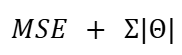
In the LASSO regularization as well, we have a hyperparameter multiplied to the penalty.

Note that both alpha and lambda represents the hyperparameter.

And as we saw in the previous blog, the theta value represents the weight of each attribute required to predict the target variable. If there is just a single attribute needed to predict the target variable, then there would be just a single theta value whereas if there are j number of attributes then the absolute of the respective theta values are summed up and multiplied by the hyperparameter.

Let’s now consider the same data points which were used in our ridge regression so that in the end it will be easier to understand what makes ridge and LASSO different from each other.

The data points in the previous blog were (0,1) and (4,9).

Let’s calculate error for the data points using the actual value and the predicted value:

The slope m is calculated by change in rise divided by change in run.

i.e ,

With our two data points (0,1) and (4,9) we can calculate the slope m.

The intercept c is calculated by substituting the x , y and m values in the equation y = mx + c

1 = 2(0) + c

The below tabular format shows the actual y (i.e y value from the data points) , the predicted y and the squared error.

The squared error is 0 and hence the MSE (Mean Squared Error) is also 0.

In the previous blog, we saw that the line of fit for this data was overfitting and the Mean Squared Error for the testing data was 14.5

As the model cannot be re-trained with extra data points, we introduced a penalty in the loss function which is the ridge regression penalty. The penalty added was the sum of the square of the theta (a value for each of the attributes). Due to this, the model adjusts the slope value to reduce overfitting and improve its ability to generalize to unseen data.

In LASSO as well, we add a penalty to the loss function, but here instead of squaring the theta value we just consider the absolute of the theta value and sum it.

But what difference does adding an absolute of the penalty and squaring of penalty make? Let’s see it now.

The test error without the penalty term was 14.5, when we add the penalty value to the loss, training loss increases because of the penalty. This often leads to better generalization on unseen test data . As we had seen that the theta value corresponds to the slope of the attributes, in our example we only have one attribute which is the line of business. Now we can assume the theta value to be the 2 as like our ridge regression example and the hyperparameter can be 10.

If we substitute these values to the loss function:

Loss = 0 + 10(2)

Loss = 20

So the loss for the training data was 0, adding the penalty to the loss becomes 20. At this stage, the model has got penalized by the penalty added, so it tries to reduce the slope value to bring down the overall loss. The model thinks that if the slope is large, I get punished. So we are penalizing large θ values inside the loss function

The new equation for the fit becomes y = 1.5x + c

Note that the slope value gets updated via the gradient descent process which is clearly explained in part 27.

For this equation, the predicted value becomes as

The MSE for the line of fit y = 1.5x + c is :

Now let’s add the penalty to this.

As usual, the training error has increased after adding the penalty term. But let’s test the new slope values for the testing data.

Now if we calculate the MSE for this data, it becomes

In the above example was just to show the behaviour of LASSO functionally. But if we observe the actual working example we can easily find the difference between LASSO and ridge. Here is an illustration:

x = 2, y = 0.5,

Let’s have the alpha value as 2.5 and the learning rate as 0.1

The optimal m value without applying LASSO regression is:

We all know that the weight updation happens via the gradient of the MSE

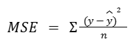
Just recollect the formula of MSE:

When we expand it , we get:

We have just replaced the predicted y with the formula of it.

Now, if we find the gradient, that is the derivative of the MSE with respect to m, we get the following:

Firstly, we differentiate it on the basis of power rule and then differentiate the internal function. So applying the power rule, it becomes:

Then we have to differentiate the y — mx+c part.

c is constant, hence it becomes 0 when we differentiate it. Differentiating mx with respect to m becomes x. y is the actual value, we find the change in MSE only by the functions involved in it.

Now, the overall derivative of the MSE becomes:

Since we have only 2 data points in our example, the 2 that appears after differentiation gets cancelled by the 2 in the denominator of the MSE formula. Therefore, we can ignore this factor and proceed with the remaining terms.

We also have to find the gradient of our penalty. The penalty for LASSO as we all know is alpha.|theta|

Here the theta is nothing but the slope value of the particular attribute. So the penalty is basically alpha.m

The gradient of the penalty term is

To be precise, the theta could be either positive or negative. Hence, the gradient of the penalty term is +alpha or -alpha

It can be re-written as:

What we can infer from this is that, when m is greater than 0, the derivative is positive. Similarly when m is negative, the derivative is negative.

With these gradients, the overall gradient of the MSE becomes:

Let’s start our calculation and let the initial slope value m be 1.

When we calculate the gradient for our example by substituting the values in the above equation, we get:

Iteration 1:

MSE gradient:

= 2×2(1×2 − 0.5) = 4(2–0.5) = 4(1.5) = 6

Penalty:

= +2.5

Total:

MSE gradient + penalty gradient

= 6+2.5 = 8.5

w = 1–0.1(8.5) = 1–0.85 = 0.15

Iteration 2:

We now use the updated weight from the first iteration.

w = 0.15

MSE:

= 2×2(0.15×2–0.5) = 4(0.3–0.5) = 4(-0.2) = -0.8

Penalty:

= +2.5

Total:

= 1.7

Update:

w = 0.15–0.17 = -0.02

Let’s do another iteration!

Iteration 3:

w = -0.02

MSE:

= 2×2(-0.02×2–0.5) = 4(-0.04–0.5) = 4(-0.54) = -2.16

Penalty:

= -2.5

Total:

= -4.66

Update:

w = -0.02 — (-0.466) = 0.446

From the three iterations, if we observe the updated weight, we get:

0.15 → -0.02 → 0.446

In our simple example that we use, we can see that the updated weight is changing between positive and negative but never reaches 0. If you continue for a few more iterations, you can observe that the updated weight value oscillates around zero but never reaches it.

This is because MSE gradient value is not strong enough to overcome the push of the penalty. If you observe carefully in each iteration , MSE gradient value is not greater than the penalty gradient value. Hence the penalty value is pushing to change the overall value back and forth from 0.

At these cases, the algorithm behind LASSO regularization works in such a way that it checks if the force of MSE gradient is strong enough to overcome the force of penalty, if it is not it locks the updated weight at 0 i.e, the gradient descent optimization process for LASSO keeps the co-efficient exactly at 0. This is the reason why LASSO regularization reaches 0 while ridge regression only nears the value 0.

LASSO regularization helps in eliminating some of the attributes by locking the updated weights of the attributes at 0. This way LASSO regularization helps in feature selection. When the coefficient of certain parameters is becoming 0, it conveys that it is not worth playing a role in predictive modelling.

In Ridge regression, the penalty term is smooth, and as the slope value approaches zero, the change in loss becomes very small. Hence, the model gradually reduces the slope but rarely makes it exactly zero.

In LASSO regression, the penalty has a sharp behavior around zero. This creates a strong push on the slope values, allowing the model to reduce them completely to zero. Once a slope becomes zero, the corresponding feature is effectively removed from the model.

Image Courtesy : ChatGPT

I hope, through this part, you were all able to understand how LASSO regularization functions and the difference between LASSO and ridge. In the next part, we shall see about Elastic Net regularization.