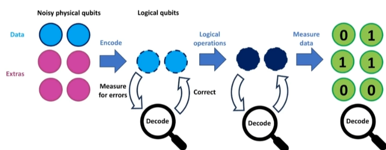
Quantum Machine Learning ( QML)

Why QML?

In classical machine learning, increasing the number of parameters leads to challenges in measuring both combined and individual contributions of features. The curse of dimensionality makes data representation and optimisation extremely difficult. Quantum Machine Learning (QML) provides a way to represent and process such high-dimensional data more efficiently by exploiting superposition, entanglement, and quantum parallelism.

QML architectures share structural similarities with classical neural networks, typically consisting of:

• Input Layer
• Processing Layer
• Output Layer
• Optimizer

Input Layer: Quantum Embedding

The role of the input layer is to convert classical data into a quantum representation, a process known as quantum embedding. Popular embedding methods include binary encoding, amplitude encoding, and angle encoding, and the choice depends on the nature of the dataset.

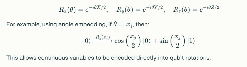
For example, in angle encoding, classical data values are mapped as rotation angles on the Bloch sphere. Quantum gates such as Rx(θ),Ry(θ), and Rz(θ) perform rotations around the respective axes, effectively embedding the input into quantum states.

Processing Layer: Quantum Transformation

The processing layer is analogous to the hidden layers in classical neural networks. Here, quantum gates transform the input states, often making use of superposition and entanglement.

Superposition is introduced using gates like the Hadamard gate (H).Entanglement can be created using gates such as CNOT or CZ.Entanglement plays a central role in capturing correlations between qubits, but not all QML architectures explicitly include it. When used, entanglement may be designed in two major structures:

Forward entanglement: where earlier layers connect progressively to later ones.

Circular entanglement: where the last layer connects back to the first layer, creating a cyclic structure.

Optimizer

Just like in classical neural networks, optimizers are used to minimize the difference between predicted and target outputs. Techniques such as gradient descent or variational quantum eigensolvers (VQEs) are employed. The optimization is often hybrid in nature: the quantum circuit generates the states, while the optimization loop uses classical computation to adjust parameters in the direction of the gradient slope for convergence to an optimal solution.