KANs: The Neural Network Revolution You Didn’t Know You Needed (Explained with Iris Classification)

A hands-on guide to Kolmogorov-Arnold Networks — the brain-inspired architecture that’s challenging everything we thought we knew about neural networks

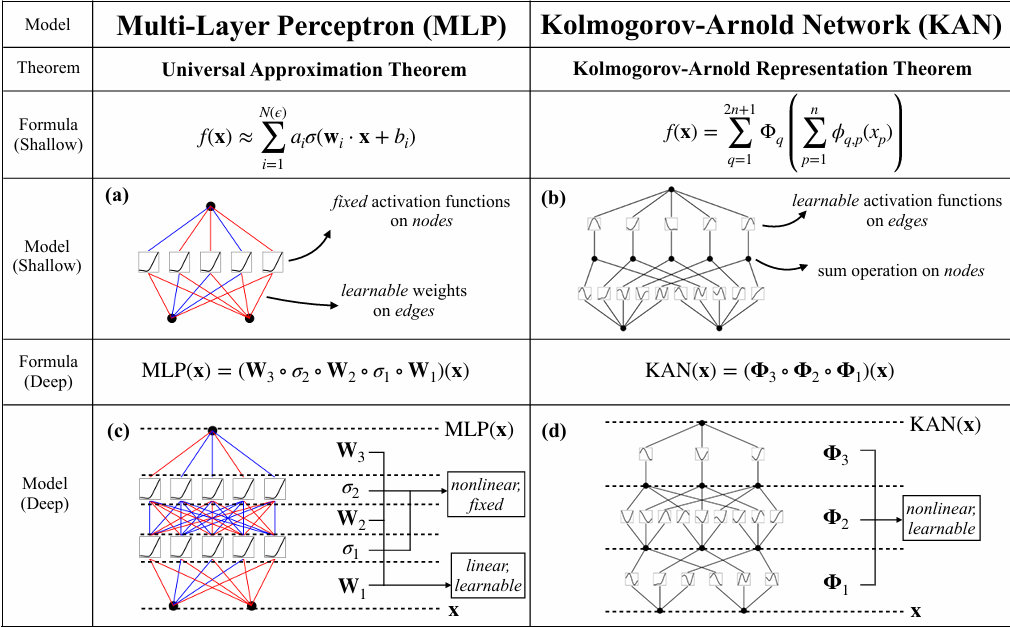
Figure: Traditional MLP (left) uses fixed activation functions on nodes, while KAN (right) learns activation functions on edges.

Remember when everyone said deep learning was just about stacking more layers and throwing more data at the problem? Well, a group of MIT researchers just dropped a paper that might change that narrative entirely.

Kolmogorov-Arnold Networks (KANs) are a fresh take on neural networks that flip the script on how we’ve been building models for decades. Instead of learning fixed weights and using predefined activation functions (like ReLU or sigmoid), KANs learn the activation functions themselves. Yes, you read that right — the activation functions are learnable.

But here’s what makes this really exciting: KANs aren’t just theoretically interesting — they’re practical, interpretable, and in many cases, more efficient than traditional MLPs (Multi-Layer Perceptrons).

In this article, I’ll walk you through KANs by building a simple classifier for the famous Iris dataset. Along the way, you’ll see why this architecture is generating so much buzz in the ML community.

In a standard neural network (MLP), each neuron does something simple:

1. Take weighted inputs
2. Sum them up
3. Apply a fixed activation function (ReLU, tanh, etc.)

The “learning” happens in the weights. The activation functions are just there to introduce non-linearity.

Output = Activation(w1*x1 + w2*x2 + ... + bias)

KANs say: “What if we put the learning on the connections (edges) instead of the nodes?”

In a KAN:

• Each edge between neurons has its own learnable function (typically a spline)
• Nodes just sum up whatever the edges send them
• No fixed activation functions anywhere

Output = φ1(x1) + φ2(x2) + ... (where each φ is learned)

This might seem like a subtle change, but it has profound implications:

1. Better Interpretability: You can actually visualize what each connection is learning
2. Smaller Models: You often need fewer parameters to achieve the same accuracy
3. Mathematical Foundation: Based on the Kolmogorov-Arnold representation theorem (we’ll get to that)

KANs are based on a mathematical result called the Kolmogorov-Arnold Representation Theorem. In simple terms, this theorem states that any continuous function of multiple variables can be written as a sum of continuous functions of single variables.

In other words: complicated multi-dimensional functions can be broken down into simpler one-dimensional pieces.

This is exactly what KANs exploit. Instead of approximating complex functions with many layers and neurons, KANs use spline functions on each edge to learn these one-dimensional mappings. Splines are just smooth, piecewise polynomial curves that can flexibly approximate almost any shape.

Think of it like this: traditional neural networks try to carve the decision space with flat planes and then stack them. KANs use flexible curves right from the start.

Enough theory — let’s see KANs in action! The Iris dataset is perfect for this because:

• It’s small (150 samples, 4 features, 3 classes)
• It’s a classic ML benchmark
• It lets us focus on the model rather than data preprocessing

Here’s where the magic happens. With pykan, creating a KAN is straightforward:

A few things to notice:

• **width**: Similar to defining layers in an MLP. We have 4 input features, 8 hidden neurons, and 3 output classes.
• **grid**: Controls the flexibility of the splines. More grid points = more flexible (but potentially overfitting).
• **k=3**: Cubic splines, which are smooth and work well in practice.

The training loop looks almost identical to any PyTorch model:

After 200 epochs, you should see accuracy climbing up to 96.67% on the test set — impressive for such a tiny model!

Here’s where KANs really shine. Unlike traditional neural networks (often called “black boxes”), KANs let you see what each connection has learned.

model(X_train) # Forward pass to set data ranges model.plot() # Visualize all edge functions

Figure: Visualization of the learned spline functions on each edge. Each subplot represents a connection in the network.

Each subplot shows what a particular edge has learned. Some might be linear, others curved, and some might be nearly flat (meaning that connection isn’t very important).

You can sharpen the visualization with:

Figure: Sharpened visualization with beta=100 for better contrast of the activation functions.

One of the coolest features is automatic pruning. KANs can identify and remove unimportant connections:

model.prune() # Marks weak edges model.plot() # Now only strong connections are visible

Figure: After pruning — weak edges are identified, revealing which connections actually matter for classification.

After pruning, you might discover that not all 4 Iris features are equally important — maybe petal length and petal width dominate the decision, while sepal dimensions play a supporting role. This is the kind of insight traditional MLPs can’t give you directly.

Figure: The final simplified network after removing pruned edges — a more compact and interpretable model.

Why KANs Might Be Better (And When They Might Not Be)

Where KANs Excel

1. Scientific Applications: When you need to understand why a model makes decisions, KANs offer symbolic regression-like interpretability. Researchers in physics and biology are particularly excited about this [1].
2. Small to Medium Datasets: With fewer samples, KANs often achieve better accuracy with fewer parameters compared to MLPs [2].
3. Function Approximation: KANs are theoretically more efficient at approximating complex functions. The original paper shows that where MLPs need O(N²) parameters, KANs might only need O(N) [2].

Where Traditional MLPs Might Still Win

1. Feature Importance: Built-in pruning tells you which inputs actually matter.
2. Large-Scale Vision/NLP: For massive models with billions of parameters, the computational overhead of splines might not be worth it (yet).
3. Highly Optimized Hardware: GPUs are incredibly optimized for matrix multiplications (the bread and butter of MLPs). Spline computations don’t benefit from these optimizations to the same degree.
4. Very Deep Networks: KANs are relatively new, and best practices for very deep KAN architectures are still being explored.

The Bigger Picture: What Does This Mean for AI?

KANs represent a philosophical shift in neural network design:

“Instead of learning fixed weights with fixed activations, learn flexible functions on the edges.”

This isn’t just about getting slightly better accuracy on benchmarks. It’s about:

1. Scientific Discovery: Models that can explain their reasoning might help scientists discover new equations and relationships in data [1].
2. Trustworthy AI: In domains like healthcare or finance, understanding why a model made a decision is just as important as the decision itself.
3. Efficiency: Smaller, pruned KANs could be easier to deploy on edge devices.

The original KAN paper from MIT is boldly titled “KAN: Kolmogorov-Arnold Networks” and makes strong claims about outperforming MLPs in terms of accuracy and interpretability [2]. While it’s still early days, the community response has been enthusiastic, with multiple implementations and extensions appearing within weeks of publication.

Try It Yourself

Getting started with KANs is easy:

$ pip install pykan

The official pykan repository has extensive documentation and tutorials. Start with a simple problem like Iris classification (as we did here), then explore more complex applications.

Key Takeaways

KANs put learnable functions on edges, not fixed activations on nodes

Based on solid math: The Kolmogorov-Arnold representation theorem

Highly interpretable: You can visualize exactly what each connection learns

Automatic pruning: Discovers which features and connections matter

Competitive accuracy: Often matches or beats MLPs with fewer parameters

Best for: Small-medium datasets, scientific applications, when interpretability matters

References

1. Liu, Z., et al. (2024). “KAN: Kolmogorov-Arnold Networks.” arXiv preprint arXiv:2404.19756. https://arxiv.org/abs/2404.19756
2. Kolmogorov, A. N. (1957). “On the representation of continuous functions of many variables by superposition of continuous functions of one variable and addition.” Doklady Akademii Nauk, 114(5), 953–956.
3. pykan GitHub Repository: https://github.com/KindXiaoming/pykan
4. Liu, Z., et al. (2024). “KAN 2.0: Kolmogorov-Arnold Networks Meet Science.” arXiv preprint arXiv:2408.10205. https://arxiv.org/abs/2408.10205
5. Hornik, K., Stinchcombe, M., & White, H. (1989). “Multilayer feedforward networks are universal approximators.” Neural networks, 2(5), 359–366.

If you found this helpful, give it a 👏 and follow for more deep dives into cutting-edge ML research!

Tags: #MachineLearning #DeepLearning #NeuralNetworks #KAN #Python #DataScience #ArtificialIntelligence

Originally published at https://github.com.