Uplift Model — targeting the right customers in Marketing Campaign

Uplift modeling, also known as incremental modeling or true lift modeling, is a predictive modeling technique used in marketing, healthcare, and other domains to estimate the causal impact of an intervention (or “treatment”) on an individual’s behavior or outcome. Unlike traditional predictive models that forecast an absolute outcome (e.g., probability of purchase), uplift models focus on the incremental effect: the difference in outcome between applying the treatment and not applying it.

Here, we will focus on a sample data curated for marketing campaigns. We generally, create predictive models with propensity to respond. Let’s understand, how we can achieve better result with a bit of different framework and do away with the traditional models.

Key Concepts:

• Potential Outcomes Framework: Rooted in causal inference (e.g., Rubin Causal Model), each individual has two potential outcomes:
• Y(1): Outcome if treated (e.g., customer receives campaign and spends $100)
• Y(0) : Outcome if not treated (e.g., same customer spends $50 without campaign)
• The individual treatment effect (ITE) or uplift is τ=Y(1)−Y(0) (e.g., +$50 incremental spend).
• In practice, we only observe one outcome per individual: Y=T⋅Y(1)+(1−T)⋅Y(0) , where T is the treatment indicator (1 = treated, 0 = control).
• Heterogeneous Treatment Effects: Uplift assumes effects vary across individuals based on features (e.g., high-recency customers may respond better to campaigns).
• Treatment Assignment: Ideally from randomized experiments (A/B tests) for unbiased estimates, but can handle observational data with adjustments (e.g., propensity scoring).
• Applications in Retail Campaigns: Identify customers where the campaign will drive incremental revenue (e.g., “persuadables”) while avoiding “sure things” (would buy anyway) or “lost causes” (won’t buy regardless). This optimizes ROI by targeting only those with positive uplift.

Suggested Framework for Customer Segmentation (Persuadables, Lost Causes, etc.)

Based on uplift modeling results, you can segment customers into four categories, as commonly used in marketing uplift applications (e.g., Lo, 2002). This framework helps prioritize campaign targeting to maximize ROI. The categories are:

1. Persuadables:

• Definition: Customers with high predicted uplift (τ=Y(1)−Y(0)>0 ), meaning they are likely to respond positively to the campaign (e.g., increase spending) but wouldn’t act without it.
• Characteristics: Often have moderate recency, frequency, or monetary values; may be “on the fence” (e.g., recency 30–60 days, moderate ATV).
• Action: Prioritize for campaign targeting (e.g., send discounts, personalized offers).
• Example: A customer with recency=45 days, frequency=5, who spends more when offered a 10% discount.

2. Sure Things:

• Definition: Customers with high baseline probability of action (Y(0) is high) and low/negative uplift, meaning they’ll act regardless of the campaign.
• Characteristics: High frequency, low recency, high loyalty scores, or high ATV.
• Action: Avoid targeting to save resources, as they don’t need incentives.
• Example: A loyal customer (recency=10 days, frequency=20) who buys regularly without discounts.

3. Lost Causes:

• Definition: Customers with low/negative uplift and low baseline action probability (Y(0)) and Y(1) both low), unlikely to respond even with the campaign.
• Characteristics: High recency (e.g., >180 days), low frequency, low monetary value.
• Action: Exclude from campaigns to avoid wasting resources.
• Example: A dormant customer (recency=300 days, frequency=1) who hasn’t purchased recently.

4. Do Not Disturbs (Sleeping Dogs):

• Definition: Customers with negative uplift (τ<0), meaning the campaign may reduce their likelihood of action (e.g., annoyance from over-targeting).
• Characteristics: May include sensitive customers or those with specific preferences (e.g., high ATV but low tolerance for frequent marketing).
• Action: Avoid targeting to prevent negative impact.
• Example: A high-value customer who reduces spending when receiving too many emails.

Common Uplift Modelling Methods:

1. S-Learner (Single Learner):

Trains one model on all data, including treatment as a feature. Uplift is predicted by setting treatment to 1 vs. 0 and taking the difference.

Model: f(X, T) → Y

Uplift = f(X, T=1) — f(X, T=0)

You predict twice per customer — once with T=1, once with T=0 — and the difference is your uplift score.

What is Y?

Y can be whatever outcome you care about, and this choice matters a lot. Common choices in retail:

1. Binary Y (most common to start)

• Did the customer purchase? (1/0)
• Did they redeem the offer? (1/0)
• Did they churn? (1/0)

In this case, f(X, T) outputs a probability, so the uplift is a probability difference:

Uplift = P(purchase | X, T=1) - P(purchase | X, T=0) e.g., 0.45–0.30 = 0.15

This customer has a 15 percentage point lift in purchase probability due to the treatment.

2. Continuous Y (revenue-based)

• Amount spent in the next 30 days
• Order value
• Number of visits

Here f(X, T) outputs a predicted spend value, so uplift becomes an incremental revenue estimate:

Uplift = ₹850 (with offer) - ₹600 (without offer) = ₹250 incremental revenue

This is more powerful for budget allocation — you can now directly compare uplift value vs. cost of the offer.

Will the Change from T=1 to T=0 Be Significant?

This is the most important practical question and the honest answer is — it depends, and often the raw difference is small but what matters is the rank-ordering.

Here’s the reality broken down:

Why the absolute difference tends to be small: The model is trained on all customers together, including Sure Things and Lost Causes. Their presence in the data “averages out” the treatment effect. A typical retail uplift score distribution might look like:

So at an individual level the numbers feel small, but the spread between customer types is what you’re exploiting.

The S-Learner specific problem:

When you have one model f(X, T) and T is just one feature among say 30 others, the model may assign T very low feature importance compared to strong signals like past purchase history or RFM. This means:

A customer with high RFM gets:

f(X, T=1) = 0.82
f(X, T=0) = 0.79 → Uplift = 0.03 (tiny, dominated by RFM signal)

Same customer via T-Learner:

f₁(X) = 0.82
f₀(X) = 0.60 → Uplift = 0.22 (treatment group model captures the actual lift)

This is exactly why S-Learner is said to underestimate uplift — the treatment variable gets shrunk relative to stronger customer features. The model “explains” most of the outcome through past behaviour, leaving little room for T to contribute.

• Pros: Simple, handles interactions via the model.
• Cons: May underperform if treatment effect is small.

2. T-Learner (Two Learners):

Trains separate models for treated and control groups. Uplift = prediction_treated — prediction_control.

Model_1: f₁(X) → Y | T=1
Model_0: f₀(X) → Y | T=0
Uplift = f₁(X) - f₀(X)

Uplift Calculation for Every Customer

Both models are trained separately, but both are applied to all 11,000 customers at inference time. (considering 11,000 customers where we need to apply, but model T =1 or T=0 have different customers). Let’s understand better!

For Customer A (was in treatment group):

f₁(A) → 0.72  (Model 1 already "saw" this type of customer)
f₀(A) → 0.48  (Model 0 predicts what A would've done without treatment)
Uplift(A) = 0.72 - 0.48 = +0.24

For Customer B (was in control group):

f₁(B) → 0.35  (Model 1 predicts what B would've done with treatment)
f₀(B) → 0.33  (Model 0 already "saw" this type of customer)
Uplift(B) = 0.35 - 0.33 = +0.02

You run both models on all 11K customers and take the difference. Every customer gets one uplift score.

Then Segmentation

Once you have 11K uplift scores, you threshold them:

• Pros: Captures group-specific patterns.
• Cons: Less efficient with small samples; no direct interaction modelling. If the treatment and control groups are imbalanced (control is small), Model_0 may be poorly estimated. The two models are trained independently so their errors don’t cancel — variance in uplift can be high. Also called the “difference of two noisy estimates” problem.

3. X-Learner (Meta-Learner):

Extends T-Learner by training meta-models on the residuals (imputed treatment effects), then combining with propensity scores.

X-Learner with 10K Treatment, 1K Control

Stage 1 — Same as T-Learner (train two base models)

f₁(X) trained on 10K treatment customers
f₀(X) trained on 1K control customers

Same as before. Same imbalance problem exists here too — but X-Learner fixes it in the next stages.

Stage 2 — Cross-Predict to Estimate Individual Treatment Effects

This is the “X” (crossing) part. Instead of directly subtracting models, you estimate what each customer’s actual personal lift was.

For treatment group (10K customers including Cust A): You already know their actual outcome Y. Use the control model f₀ to ask — “what would A have done without treatment?”

τ₁(A) = Y_actual(A) - f₀(A)
      = 1 (purchased) - 0.48 (control model prediction) = +0.52

This is A’s estimated personal uplift. Do this for all 10K treatment customers.

For control group (1K customers including Cust B): You already know their actual outcome Y. Use the treatment model f₁ to ask — “what would B have done if treated?”

τ₀(B)  = f₁(B) - Y_actual(B)
       = 0.35 (treatment model prediction) - 0 (didn't purchase) = +0.35

Do this for all 1K control customers.

Now you have estimated ITE (Individual Treatment Effect) for every customer in their respective groups.

Stage 3 — Train Two More Models on These ITEs

Going back to Stage 2, you computed a numeric ITE value for every customer:

Treatment group (10K): τ₁(A) = Y_actual - f₀(A) = 1 - 0.48 = +0.52
Control group (1K):    τ₀(B) = f₁(B) - Y_actual = 0.35 - 0 = +0.35

These τ values are continuous numbers (can be negative, zero, positive). So Stage 3 is purely regression, not classification.

Model_τ₁: trained on 10K treatment customers → predicts τ₁
Model_τ₀: trained on 1K control customers   → predicts τ₀

These models learn which features drive the uplift, not just the outcome.

The training data for each model looks like this:

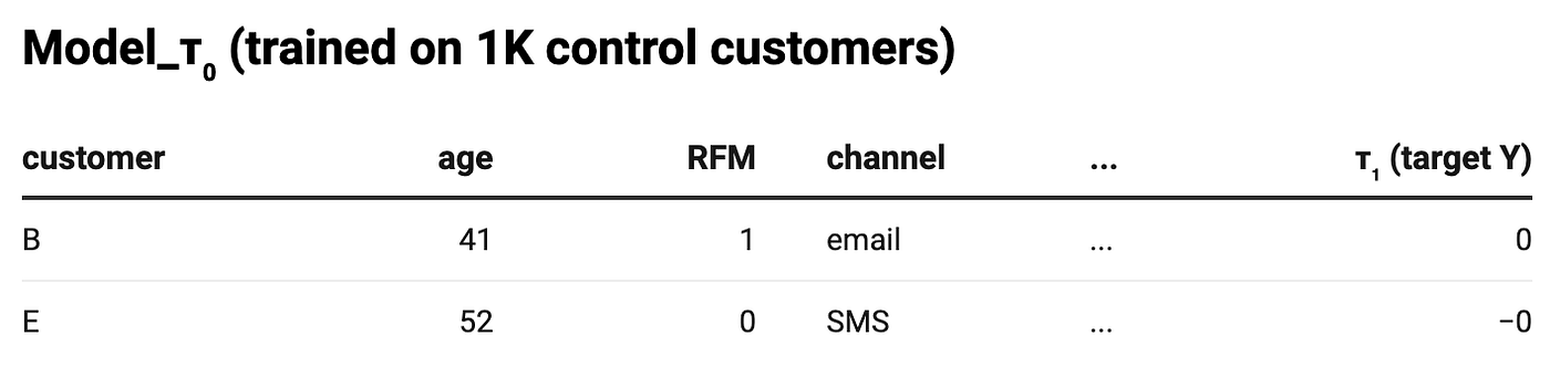
So X (features) are the same customer attributes. Y is the ITE estimate from Stage 2. The model is learning which customer characteristics predict a high or low treatment effect — not which customers buy, but which customers respond incrementally.

Where Does e(X) Come From?

e(X) is a separate fifth model — a propensity model — trained on your entire 11K population:

This is a binary classification model. Y here is simply whether the customer was in treatment or control. Output is a probability — P(T=1 | X).

With 10K treated and 1K control, most customers look like treated customers, so e(X) will be high for most people — say 0.85 to 0.95.

Stage 4 — Combine Using Propensity Score

Train a propensity model e(X) = P(T=1 | X). With 10K treatment and 1K control, most customers will have high propensity scores (model knows treatment was dominant).

Uplift(A) = e(X) × τ₀(A)  +  (1 - e(X)) × τ₁(A)

Why this weighting matters with 10K/1K imbalance:

Since 10K were treated, e(X) for most customers will be high (say 0.9). This means:

Uplift = 0.9 × τ₀  +  0.1 × τ₁

It leans heavily on τ₀ — the model trained on control data. This is intentional. With only 1K control customers, each one carries more signal about the counterfactual, so X-Learner up weights that signal. It’s essentially saying “the rare control customers tell us more about what would have happened without treatment.”

Putting It Together for Customer A

At inference time, you run all five models on A’s features:

Stage 3 models give:
  Model_τ₁(A) → predicts A's uplift from treatment-group perspective = 0.52
  Model_τ₀(A) → predicts A's uplift from control-group perspective  = 0.41

Propensity model gives:
e(A) = 0.90  (90% chance A would be in treatment, given the 10:1     ratio)

Final Uplift(A) = e(X) × τ₀(A) +  (1 - e(X)) × τ₁(A)
                = 0.90 × 0.41  +  0.10 × 0.52
                = 0.369        +  0.052
                = 0.42

Because e(X) = 0.90, the formula trusts τ₀ more — the estimate derived from the scarce 1K control group — because those customers represent the rare counterfactual signal. The 10K treatment group is abundant, so it needs less weight.

All 5 Models Summary

• Pros: Robust to imbalanced treatment; good for heterogeneous effects.
• Cons: More complex.

4. Other Advanced Methods:

Uplift trees/forests (decision trees splitting on uplift), causal forests, or neural network-based approaches. Evaluation often uses QINI (Quality of Incremental Net Information) or AUUC (Area Under Uplift Curve) to compare models, plotting cumulative uplift vs. proportion targeted.

Let’s take a deep dive into the python code with simulated data. Generated the data with RFM features, with base spend and uplift f

# Set seed for reproducibility
np.random.seed(42)

# Generate synthetic transaction data
num_customers = 500
customer_ids = np.arange(1, num_customers + 1)
current_date = datetime(2025, 10, 1)

# For each customer, generate 1-20 transactions over last 5 years
transactions = []
for cid in customer_ids:
    num_trans = np.random.randint(1, 21)
    dates = [current_date - timedelta(days=np.random.randint(1, 1826)) for _ in range(num_trans)]
    amounts = np.random.uniform(10, 500, num_trans)
    for d, a in zip(dates, amounts):
        transactions.append({'customer_id': cid, 'purchase_date': d, 'amount': a})

df_trans = pd.DataFrame(transactions)

# Compute RFM per customer
df_rfm = df_trans.groupby('customer_id').agg(
    last_purchase=('purchase_date', 'max'),
    frequency=('amount', 'count'),
    monetary=('amount', 'sum')
).reset_index()

df_rfm['recency'] = (current_date - df_rfm['last_purchase']).dt.days
df_rfm['atv'] = df_rfm['monetary'] / df_rfm['frequency']

# Add other features
df_rfm['age'] = np.random.randint(18, 71, num_customers)
df_rfm['gender'] = np.random.choice(['M', 'F'], num_customers)
df_rfm['loyalty_score'] = np.random.uniform(0, 1, num_customers)

# Ensure index aligns and fill NaNs if any
df_rfm = df_rfm.set_index('customer_id').reindex(customer_ids).reset_index().fillna(0)

# Simulate treatment (campaign sent, randomized)
df_rfm['treatment'] = np.random.binomial(1, 0.5, num_customers)# Simulate outcomes with heterogeneous uplift
base_spend = 0.5 * df_rfm['monetary'] + np.random.normal(0, 50, num_customers)
uplift = 20 * (df_rfm['recency'] < 60) + 10 * (df_rfm['frequency'] > 10) + np.random.normal(0, 5, num_customers)
y1 = base_spend + uplift
y0 = base_spend
df_rfm['outcome'] = df_rfm['treatment'] * y1 + (1 - df_rfm['treatment']) * y0
df_rfm['true_uplift'] = uplift

However, in a real dataset (e.g., from a retail CRM system with transaction logs), we don’t directly “find” or compute these values the same way. Instead:

• base_spend approximates the counterfactual outcome Y(0) (what would happen without treatment/campaign).
• uplift estimates the individual treatment effect τ=Y(1)−Y(0) (incremental impact of the campaign).

These rely on assumptions grounded in domain knowledge (e.g., recent/low-frequency customers respond better to campaigns), but everything ultimately depends on data quality and experimental design. Below, I’ll explain the theory, how to derive them in real data, and key assumptions.

Data snapshot.

# Features for modeling
features = ['recency', 'frequency', 'monetary', 'atv', 'age', 'loyalty_score']
X = df_rfm[features]
X = pd.concat([X, pd.get_dummies(df_rfm['gender'], prefix='gender', dtype=int)], axis=1)
X = X.astype(float)  # Force numeric dtypes
y = df_rfm['outcome'].astype(float)
treatment = df_rfm['treatment'].astype(float)
true_uplift = df_rfm['true_uplift'].astype(float)

# Manual split
X_train, X_test, y_train, y_test = manual_train_test_split(X, y, test_size=0.2)
treat_train = treatment.iloc[X_train.index].astype(float)
treat_test = treatment.iloc[X_test.index].astype(float)
true_uplift_test = true_uplift.iloc[X_test.index].astype(float)

# Simplified AUUC computation
def compute_auuc(y_true_uplift, y_pred_uplift):
    sorted_idx = np.argsort(-y_pred_uplift)
    cum_uplift = np.cumsum(y_true_uplift.iloc[sorted_idx]) / np.arange(1, len(y_true_uplift) + 1)
    auuc = np.trapz(cum_uplift, dx=1.0 / len(y_true_uplift))
    return auuc, cum_uplift

# S-Learner
X_s_train = pd.concat([X_train.reset_index(drop=True), treat_train.reset_index(drop=True).rename('treatment')], axis=1)
X_s_train_const = sm.add_constant(X_s_train)
model_s = sm.OLS(y_train.reset_index(drop=True).values, X_s_train_const.values).fit()

# Manual construction for test exog to ensure consistent columns and dtypes
const_df = pd.DataFrame({'const': 1.0}, index=X_test.index)
treat_df_1 = pd.DataFrame({'treatment': 1.0}, index=X_test.index)
treat_df_0 = pd.DataFrame({'treatment': 0.0}, index=X_test.index)
X_test_const_1 = pd.concat([const_df, X_test, treat_df_1], axis=1).astype(float)
X_test_const_0 = pd.concat([const_df, X_test, treat_df_0], axis=1).astype(float)
uplift_s = model_s.predict(X_test_const_1.values) - model_s.predict(X_test_const_0.values)

# T-Learner
train_t_mask = treat_train == 1
train_c_mask = ~train_t_mask
X_train_t = X_train[train_t_mask]
y_train_t = y_train[train_t_mask]
X_train_c = X_train[train_c_mask]
y_train_c = y_train[train_c_mask]

X_train_t_const = sm.add_constant(X_train_t.reset_index(drop=True))
model_t = sm.OLS(y_train_t.reset_index(drop=True).values, X_train_t_const.values).fit()
X_train_c_const = sm.add_constant(X_train_c.reset_index(drop=True))
model_c = sm.OLS(y_train_c.reset_index(drop=True).values, X_train_c_const.values).fit()

X_test_const = sm.add_constant(X_test.reset_index(drop=True))
uplift_t = model_t.predict(X_test_const.values) - model_c.predict(X_test_const.values)

# X-Learner (fixed residuals)
pred_c_on_t = model_c.predict(sm.add_constant(X_train_t.reset_index(drop=True)).values)
d_train_t = y_train_t.reset_index(drop=True) - pred_c_on_t
pred_t_on_c = model_t.predict(sm.add_constant(X_train_c.reset_index(drop=True)).values)
d_train_c = pred_t_on_c - y_train_c.reset_index(drop=True)

X_train_t_const_meta = sm.add_constant(X_train_t.reset_index(drop=True))
model_mt = sm.OLS(d_train_t.values, X_train_t_const_meta.values).fit()
X_train_c_const_meta = sm.add_constant(X_train_c.reset_index(drop=True))
model_mc = sm.OLS(d_train_c.values, X_train_c_const_meta.values).fit()

prop = treat_train.mean()
uplift_x = prop * model_mt.predict(X_test_const.values) + (1 - prop) * model_mc.predict(X_test_const.values)

Evaluation:

• Uplift Curve: Sort customers by predicted uplift (descending), plot cumulative incremental outcome vs. % targeted.
• QINI Coefficient: Area between uplift curve and random targeting line, normalized.
• Challenges: Selection bias, confounding, need for validation (e.g., holdout set).

# Evaluations
mae_s = manual_mae(true_uplift_test, uplift_s)
mae_t = manual_mae(true_uplift_test, uplift_t)
mae_x = manual_mae(true_uplift_test, uplift_x)
print(f"MAE S-Learner: {mae_s:.2f}")
print(f"MAE T-Learner: {mae_t:.2f}")
print(f"MAE X-Learner: {mae_x:.2f}")

auuc_s, cum_s = compute_auuc(true_uplift_test, uplift_s)
auuc_t, cum_t = compute_auuc(true_uplift_test, uplift_t)
auuc_x, cum_x = compute_auuc(true_uplift_test, uplift_x)
print(f"AUUC S-Learner: {auuc_s:.4f}")
print(f"AUUC T-Learner: {auuc_t:.4f}")
print(f"AUUC X-Learner: {auuc_x:.4f}")

MAE S-Learner: 11.01
MAE T-Learner: 15.49
MAE X-Learner: 15.49
AUUC S-Learner: 8.4937
AUUC T-Learner: 12.1145
AUUC X-Learner: 12.1145

# Plots
fig, axs = plt.subplots(1, 2, figsize=(15, 6))

# 1. Uplift Distribution
axs[0].hist(uplift_s, alpha=0.5, label='S-Learner', bins=20)
axs[0].hist(uplift_t, alpha=0.5, label='T-Learner', bins=20)
axs[0].hist(uplift_x, alpha=0.5, label='X-Learner', bins=20)
axs[0].hist(true_uplift_test, alpha=0.5, label='True Uplift', bins=20)
axs[0].legend()
axs[0].set_title('Distribution of Predicted vs True Uplift')

# 2. Uplift Curves
prop_targeted = np.linspace(0, 1, len(cum_s))
axs[1].plot(prop_targeted, cum_s, label='S-Learner')
axs[1].plot(prop_targeted, cum_t, label='T-Learner')
axs[1].plot(prop_targeted, cum_x, label='X-Learner')
axs[1].plot([0, 1], [0, true_uplift_test.mean()], 'k--', label='Random')
axs[1].legend()
axs[1].set_title('Uplift Curves')
axs[1].set_xlabel('Proportion Targeted')
axs[1].set_ylabel('Cumulative Average Uplift')

plt.tight_layout()
plt.show()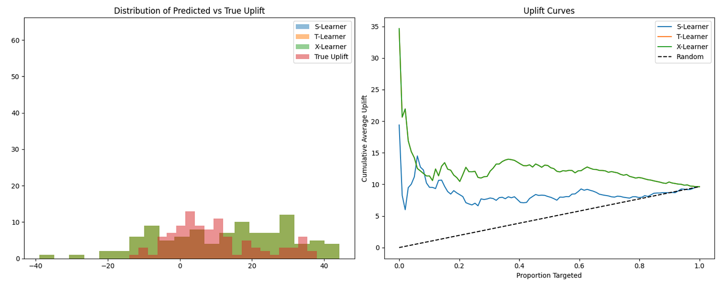

# Target customers: top 20% by average uplift
avg_uplift = (uplift_s + uplift_t + uplift_x) / 3
df_test = df_rfm.loc[X_test.index].copy()
df_test['pred_uplift'] = avg_uplift
target_customers = df_test.sort_values('pred_uplift', ascending=False).head(int(0.2 * len(X_test)))
print("\nTop Customers to Target:")
print(target_customers[['customer_id', 'recency', 'frequency', 'monetary', 'atv', 'pred_uplift']])

Top Customers to Target:
     customer_id  recency  frequency     monetary         atv  pred_uplift
211          212       56         18  3420.499751  190.027764    33.935191
9             10      190         12  2675.153864  222.929489    33.282486
381          382       45         17  4632.240935  272.484761    33.069031
333          334      449         14  3851.599957  275.114283    32.248652
324          325      214         20  4599.647878  229.982394    30.083283
15            16      161         18  4425.022071  245.834559    29.910347
414          415      126         11  2860.579992  260.052727    29.230422
317          318      393         18  4598.989879  255.499438    28.857276
450          451      143         18  4094.977352  227.498742    28.783513
148          149       68         16  4286.561981  267.910124    28.286999
277          278       83         19  5717.905414  300.942390    26.540648
451          452     1051          5   730.555049  146.111010    26.401635
18            19       51         16  4061.857568  253.866098    25.708200
90            91      361         16  4560.953759  285.059610    25.179615
73            74       17         12  2480.938248  206.744854    24.480575
341          342       31          9  2062.671932  229.185770    24.447954
238          239      125          9  1974.264594  219.362733    24.073120
0              1      861          7  1327.362051  189.623150    23.903983
312          313       69         17  5202.830690  306.048864    23.671902
193          194      295         19  4851.073024  255.319633    23.508695

Let’s take a look into few advanced techniques.

Causal Random Forests (Causal RF) and EconML

Causal Random Forests (Causal RF) and EconML are advanced tools for uplift modeling and causal inference, particularly for estimating heterogeneous treatment effects in applications like retail campaign targeting. Below is a detailed comparison, followed by a suggested framework for categorising customers (e.g., persuadables, lost causes) based on uplift modeling results.

Comparison: Causal Random Forests vs. EconML

1. Overview

• Causal Random Forests:
• A tree-based method extending random forests to estimate individual treatment effects (ITE) or uplift. It splits data to maximise heterogeneity in treatment effects rather than just outcome variance.
• Often implemented via libraries like causalml (Python) or grf (R, Generalized Random Forests).
• Focuses on non-parametric estimation, making it flexible for complex, non-linear relationships.
• EconML:
• A Python library developed by Microsoft Research for causal inference, offering a suite of methods for estimating conditional average treatment effects (CATE).
• Includes multiple algorithms: Double Machine Learning (DML), Causal Forest, Deep IV, DRLearner, etc.
• Combines machine learning with econometric principles, allowing for both parametric and non-parametric approaches.

2. Methodology

• Causal RF:
• Core Idea: Modifies decision tree splits to optimize for differences in treatment effects across subgroups, using criteria like expected uplift variance.
• Key Algorithms:
• Uplift Random Forests (e.g., in causalml) use divergence measures (e.g., KL-divergence, Euclidean distance) to split nodes based on uplift.
• Generalized Random Forests (grf) estimate CATE via honest splitting (separating tree-building and estimation data).
• Strengths:
• Handles non-linear relationships and interactions well.
• Robust to high-dimensional data.
• Interpretable through feature importance and tree structures.
• Weaknesses:
• Computationally intensive for large datasets.
• May overfit without careful tuning (e.g., min samples per leaf, depth).
• Limited to tree-based modeling, which may not capture all patterns as effectively as neural methods.
• EconML:
• Core Idea: Leverages a variety of machine learning models (e.g., linear, tree-based, neural) within econometric frameworks to estimate CATE, often correcting for confounding using propensity scores or instrumental variables.
• Key Algorithms:
• Double Machine Learning (DML): Combines two models (one for outcome, one for treatment) to remove bias from confounding, using flexible ML models (e.g., XGBoost, neural nets).
• Causal Forest: Similar to Causal RF but integrated with DML for robustness.
• Deep IV: Uses neural networks for instrumental variable estimation.
• DRLearner: Combines DML with regression adjustment for small treatment effects.
• Strengths:
• Highly flexible: supports multiple base learners (e.g., linear, gradient boosting, neural nets).
• Handles confounding rigorously via econometric methods.
• Scales to complex datasets and offers methods for both randomized and observational data.
• Weaknesses:
• More complex to set up (requires specifying nuisance models, e.g., propensity).
• Computationally heavy for some methods (e.g., Deep IV).
• Less interpretable for non-tree-based methods (e.g., neural nets).

With the above sample generated data, here is the extension of the code using CausalMl and EconML.

# CausalML Uplift (meta-learner for regression)
causal_model = XGBTRegressor(random_state=42, n_estimators=100, max_depth=5)
causal_model.fit(X_train.values, treat_train.values, y_train.values)
uplift_causal_raw = causal_model.predict(X_test.values)
uplift_causal = np.mean(uplift_causal_raw, axis=1)  

# EconML Causal Forest DML 
econml_model = CausalForestDML(
    model_y=xgb.XGBRegressor(random_state=42),
    model_t=xgb.XGBClassifier(random_state=42),
    n_estimators=100, max_depth=5, min_samples_leaf=5, random_state=42,
    discrete_treatment=True  
)
econml_model.fit(Y=y_train.values, T=treat_train.values, X=X_train.values)
uplift_econml = econml_model.effect(X_test.values)

# Evaluations
mae_causal = manual_mae(true_uplift_test, uplift_causal)
mae_econml = manual_mae(true_uplift_test, uplift_econml)
print(f"MAE CausalML XGBTRegressor: {mae_causal:.2f}")
print(f"MAE EconML: {mae_econml:.2f}")

auuc_causal, cum_causal = compute_auuc(true_uplift_test, uplift_causal)
auuc_econml, cum_econml = compute_auuc(true_uplift_test, uplift_econml)
print(f"AUUC CausalML: {auuc_causal:.4f}")
print(f"AUUC EconML: {auuc_econml:.4f}")

MAE CausalML XGBTRegressor: 14.31
MAE EconML: 9.92
AUUC CausalML: 9.7497
AUUC EconML: 11.3211

# Plot Uplift Curves
prop_targeted = np.linspace(0, 1, len(cum_causal))
plt.figure(figsize=(10, 6))
plt.plot(prop_targeted, cum_causal, label='CausalML XGBTRegressor')
plt.plot(prop_targeted, cum_econml, label='EconML Causal Forest')
plt.plot([0, 1], [0, true_uplift_test.mean()], 'k--', label='Random')
plt.legend()
plt.title('Uplift Curves: CausalML vs EconML')
plt.xlabel('Proportion of Population Targeted')
plt.ylabel('Cumulative Average Uplift')
plt.show()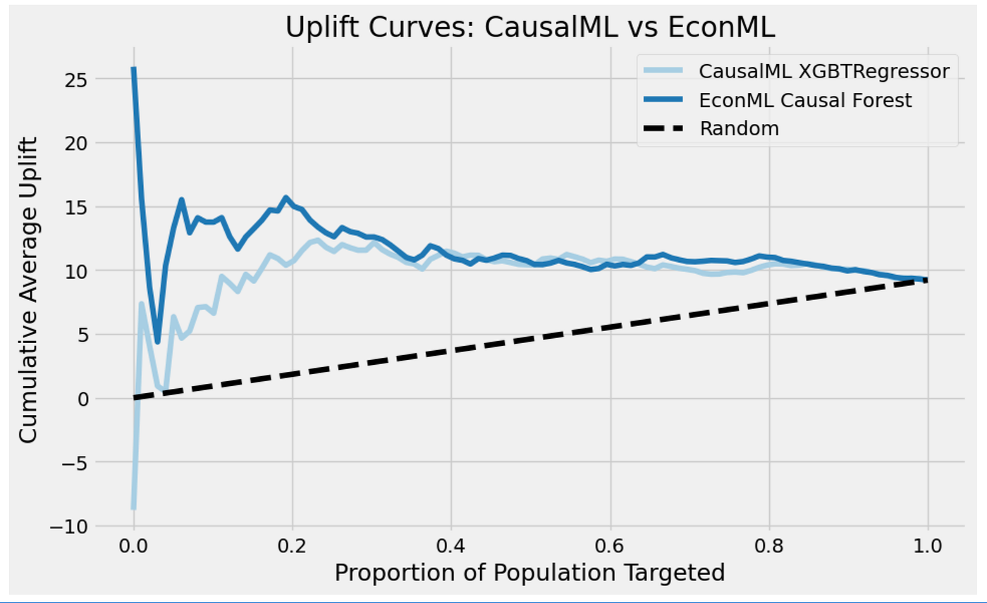

Customer Segmentation Summary:

# Categorize
quantiles = df_test['pred_uplift'].quantile([0.25, 0.75])
q_low, q_high = quantiles[0.25], quantiles[0.75]
baseline_threshold = df_test['baseline_outcome'].quantile(0.5)

def categorize_customer(row):
    uplift = row['pred_uplift']
    baseline = row['baseline_outcome']
    if uplift > q_high and baseline < baseline_threshold:
        return 'Persuadable'
    elif uplift < q_low and baseline < baseline_threshold:
        return 'Lost Cause'
    elif uplift < q_low and baseline >= baseline_threshold:
        return 'Sure Thing'
    else:
        return 'Do Not Disturb'

df_test['category'] = df_test.apply(categorize_customer, axis=1)

print("\nCustomer Segmentation Summary:")
print(df_test.groupby('category').size())

print("\nTop Persuadables:")
print(df_test.query("category == 'Persuadable'")[['customer_id', 'recency', 'frequency', 'monetary', 'atv', 'pred_uplift']].head())

Customer Segmentation Summary:
category
Do Not Disturb    66
Lost Cause        17
Persuadable        9
Sure Thing         8
dtype: int64

Top Persuadables:
     customer_id  recency  frequency     monetary         atv  pred_uplift
124          125      238          8  2515.487251  314.435906    38.552566
194          195      121          6  1420.552104  236.758684    35.726263
490          491      311          3   194.882032   64.960677    83.425751
93            94       21         11  2517.850317  228.895483    63.887525
185          186     1015          3   810.209238  270.069746    62.505747

How to Derive These in Real Data

In practice, you use historical data from A/B tests (randomized campaigns) or observational data (past promotions with propensity score matching to mimic randomization). Here’s a step-by-step adaptation:

1. Prepare Real Data:

• Start with transaction logs (like df_trans in the code): customer_id, purchase_date, amount.
• Compute RFM + extras (recency, frequency, monetary, ATV, demographics).
• Add a treatment column: Binary flag for exposure to a past campaign (e.g., email sent = 1).
• Add outcome: e.g., spend in a post-campaign window (e.g., next 30 days).

2. Estimate base_spend (Y(0)):

• From control group (T=0): Average/median spend, adjusted for features.
• Real formula: Use a model (e.g., linear regression) on control data:

• Why not direct average? To account for heterogeneity (e.g., high-monetary customers spend more baseline).
• In code: Fit an OLS on control subsample, predict for all customers.

3. Estimate uplift (τ):

• Use uplift models (as in our code: S/T/X-Learners, Causal RF, EconML) on full data.
• These implicitly learn relationships like “low recency → +20 uplift” from treated vs. control differences.
• No explicit formula like the synthetic one — instead, the model discovers coefficients/patterns.
• Validation: Use QINI/AUUC on a holdout set; run new A/B tests to confirm.

4. Incorporate Domain Assumptions:

• The synthetic uplift assumes: Recent customers (<60 days) get +20 (they’re “warm” leads); high-frequency (>10) get +10 (loyal but need nudge).
• In real data: Hypothesize based on business logic (e.g., from past campaigns: “dormant users uplift 15–25%”). Test via feature importance in models.