Exploring the Core Mechanics of CPU Scheduling Algorithms

Understanding CPU Scheduling:

CPU Scheduling is the process used by an Operating System (OS) to decide which process or task should be given access to the CPU next. Since a CPU can execute only one process at a time (in a single-core system), but multiple processes are waiting to run, the OS uses scheduling algorithms to manage this competition.

In simple words, CPU Scheduling ensures that every process gets a fair chance to run while maximizing the overall performance of the system.

It helps the OS to:

Improve CPU efficiency

Reduce waiting time

Increase system responsiveness

Allow multitasking

Prevent a single process from blocking the entire system

CPU Scheduling plays a central role in process management and is essential for achieving smooth, fast, and stable system performance.

Preemptive vs Non-Preemptive Scheduling: Key Differences:

This distinction is key to understanding schedulers.

Non-Preemptive Scheduling (Cooperative Scheduling)

In non-preemptive scheduling, once a process gets the CPU, it retains it until one of the following occurs:

• The process finishes its execution
• The process voluntarily releases the CPU (e.g., waiting for I/O)
• The process terminates

Key Features:

• Easy to implement — Kernel code is less complex
• Lower overhead — Fewer context switches
• Predictable behavior — Control returns at known times
• Risk of CPU monopolization — A long process may block others

Analogy:

Think of it like giving someone the microphone in a meeting — they speak until they finish, no matter how long it takes.

Preemptive Scheduling

In preemptive scheduling, the operating system can interrupt a running process and assign the CPU to another process. This can occur when:

• A timer expires (time quantum is over)
• A higher-priority process arrives
• A process with shorter remaining time arrives

Key Features:

• Better responsiveness — Ideal for interactive applications
• Fair CPU allocation — No single process can hog the CPU
• Higher overhead — More frequent context switches
• More complex implementation — Requires careful synchronization

Analogy:

Think of it like a meeting moderator who can interrupt long-winded speakers to allow others a turn.

Algorithms Supporting Both Modes:

Some scheduling algorithms, such as Shortest Job Next (SJN) and Priority Scheduling, can operate in both preemptive and non-preemptive modes. FCFS usually works non-preemptively, while Round Robin is inherently preemptive.Certain algorithms like SJN and Priority Scheduling are flexible and can function in either mode. In contrast, FCFS is typically non-preemptive, and Round Robin always uses preemption.

Algorithms No:01:

FCFS Scheduling in OS: Examples & Gantt Chart:

1. Introduction

FCFS Scheduling follows a first-come, first-served principle. The CPU is allocated to the process that has been waiting the longest, and it continues running until the process finishes.

Analogy:

Think of it like a ticket counter at a train station — first person in line gets the ticket first, and no one can jump the queue.

Key Features of FCFS Scheduling

• Scheduling Type: Non-preemptive — Once a process begins, it runs until it finishes, no interruptions.
• Queue Implementation: Processes are handled in a FIFO (First-In, First-Out) manner, like a line at a counter.
• Simplicity: Very straightforward to understand and code, making it beginner-friendly.
• Limitation: If a long process arrives first, it can cause other processes to wait longer, increasing average waiting time.

Analogy:

Think of it like a queue at a bakery: whoever joins first, gets served first, but if the first person orders a large cake, everyone else waits longer.

Important Terms in FCFS Scheduling

• Arrival Time (AT): The time at which a process enters the ready queue.
• Burst Time (BT): The total CPU time required by a process to complete execution.
• Completion Time (CT): The time at which a process finishes execution.
• Turnaround Time (TAT): The total time a process spends in the system. Formula: TAT = Completion Time − Arrival Time
• Waiting Time (WT): The total time a process spends waiting in the ready queue. Formula: WT = Turnaround Time − Burst Time

Additional Info:

• Scheduling Criteria: Based on Arrival Time
• Mode: Non-preemptive

FCFS Scheduling Example:

Scheduling Type: Non-preemptive (FCFS) Criteria: Arrival Time

Tasks to Compute in FCFS Scheduling

When solving an FCFS scheduling example, you should compute the following:

1. Draw the Gantt Chart

• Show the order of process execution
• Include any idle CPU slots if they exist

2. Determine Completion Time (CT)

• The time when each process finishes execution

3. Calculate Turnaround Time (TAT)

• Formula: TAT = CT − AT
• Total time a process spends in the system

4. Calculate Waiting Time (WT)

• Formula: WT = TAT − BT
• Time a process spends waiting in the ready queue

5. Compute Average TAT and Average WT

• Average values for all processes

6. Calculate CPU Utilization

• Formula: CPU Utilization = (Busy Time / Total Time) × 100%
• Measures how efficiently CPU is being used

Gantt chart:

Calculations:

CPU Utilization

Step 1: Calculate Total Busy Time

• Add up the Burst Times (BT) of all processes:
• Total Busy Time=6+4+1+3+5+2=21\text{Total Busy Time} = 6 + 4 + 1 + 3 + 5 + 2 = 21Total Busy Time=6+4+1+3+5+2=21

Step 2: Calculate Total Time Span

• From start of first process (0) to completion of last process (21):
• Total Time=21\text{Total Time} = 21Total Time=21

Step 3: Compute CPU Utilization

CPU Utilization=Total Busy TimeTotal Time×100%=2121×100%=100%\text{CPU Utilization} = \frac{\text{Total Busy Time}}{\text{Total Time}} \times 100\% = \frac{21}{21} \times 100\% = 100\%CPU Utilization=Total TimeTotal Busy Time​×100%=2121​×100%=100%

Observation:

• There were no idle slots in this example.
• The CPU remained busy throughout, achieving 100% utilization.

CPU Idle Time (Idle Slot)

Alternative Title Options:

1.CPU Idle Time Explained

2. Understanding Idle Slots in Scheduling

3. When CPU Remains Idle

4. Idle Periods in CPU Scheduling

Step 1: Definition

• Idle Slot / CPU Idle Time is the period when the CPU has no process to execute, remaining unoccupied.

Step 2: When It Occurs

• Happens when the next process in the ready queue arrives after the current process completes.
• Example:
• Process P1 finishes at t = 10
• Next process P2 arrives at t = 12
• CPU remains idle for 12 − 10 = 2 units of time

Step 3: Significance

• Idle time is undesirable because it represents wasted CPU cycles.
• Scheduling algorithms aim to minimize or eliminate idle periods, keeping the CPU continuously busy.

FCFS Scheduling Example with CPU Idle Time:

• Scheduling Criteria: Arrival Time (AT)
• Mode: Non-preemptive

Gantt Chart:

The Gantt Chart shows the order of process execution and highlights any idle slots when the CPU is not running a process.

CPU Scheduling Performance Metrics:

FCFS Scheduling When Arrival Time Is Missing:

Scenario: Arrival Time Not Provided

• Assumption: All processes have Arrival Time (AT) = 0 by default.
• What This Means:
• All processes are present in the ready queue at time 0.
• FCFS executes processes in the order they appear, ignoring arrival times.
• Illustrative Example:

Execution Sequence: P1 → P2 → P3

• Each process starts as soon as the previous one finishes.
• No arrival times are needed for computation.

Case 2: Arrival Time = 0 for All Processes

• Scenario: All processes have AT = 0, meaning they arrive simultaneously at the ready queue.
• Implications:

1. FCFS executes processes in the order they appear in the list.
2. There is no CPU idle time — the CPU is continuously busy.
3. This is considered the simplest form of FCFS scheduling.

Scheduling Type: Non-preemptive (FCFS) Criteria: Arrival Time (all 0)

Advantages of FCFS:

• Simple to implement — easy to code and understand
• Fair scheduling — no process starvation
• Beginner-friendly — ideal for learning CPU scheduling concepts

Disadvantages of FCFS:

• High average waiting time — especially with long processes
• Convoy effect — short processes get delayed behind long ones
• Not suitable for time-sharing systems — poor responsiveness
• Slow response time — affects interactive applications

Real-Life Analogy of FCFS

• Scenario: People lining up at a ticket counter or checkout queue
• FCFS Analogy: The person who arrives first is served first
• Takeaway: Shows the first-come-first-served principle applied in daily life

Practical Applications of FCFS

• Batch processing systems — where tasks are executed sequentially
• Simple, non-interactive operations — no urgent response needed
• Fair scheduling scenarios — all processes treated equally
• Processes of equal importance — avoids prioritization conflicts

Key Questions to Explore

1. Execution Timing: When does each process get the CPU?
2. CPU Idle Behavior: What does the CPU do when no process is ready?
3. Efficiency Metrics: Why are lower Waiting Time (WT) and Turnaround Time (TAT) desirable?

ALgorithm : No:02:

Understanding Shortest Remaining Time First (SRTF) Scheduling

Also Called: Preemptive Shortest Job First (SJF)

SRTF is a preemptive CPU scheduling algorithm that always picks the process with the shortest remaining execution time. It helps reduce average waiting time compared to non-preemptive algorithms, but it requires careful tracking of remaining times.

How SRTF Scheduling Works Step by Step

Constantly Checking the Ready Queue

The CPU keeps checking the ready queue at every time unit to see if a new process has arrived.

Selecting the Process with Least Remaining Time

At any time, the CPU runs the process that has the smallest remaining burst time.

Interrupting the Running Process (Preemption)

If a new process arrives with less remaining time than the current process, the CPU switches immediately to the new process.

Running Processes One Unit at a Time

• Think of the CPU as running one unit of time for a process.
• After each unit, the scheduler checks:

1. Has a new process arrived?
2. Which process now has the shortest remaining time?
3. How much time is left for the currently running process?

• The CPU is then assigned to the process with the least remaining time.

Key Points:

• SRTF is dynamic and preemptive.
• Minimizes average waiting time.
• More complex to implement than non-preemptive algorithms.
• Best for interactive and batch systems where responsiveness matters.

Handling Edge Cases in SRTF: Tie-Breaking Rules

In SRTF scheduling, it’s common for two or more processes to have the same shortest remaining burst time. To maintain a consistent and predictable schedule, tie-breaking rules are applied.

1. Arrival Time (AT) Priority

• If multiple processes share the same shortest remaining time, the CPU is given to the process that arrived first (smallest AT).
• This ensures that earlier processes are favored when ties occur.

2. Process ID (PID) Priority

• If both the remaining burst time and arrival time are identical, the CPU is assigned to the process with the smallest Process ID (PID).
• This guarantees a deterministic and consistent decision every time a tie occurs.

Why SRTF Is Efficient Despite Its Complexity

SRTF is more complicated than other scheduling algorithms because:

• The CPU has to constantly switch between processes (preemption).
• It needs to keep track of the remaining burst time of every process.

However, this extra effort makes it very effective:

• By always choosing the process with the shortest remaining time, SRTF minimizes average waiting time.
• This makes it one of the most efficient scheduling algorithms when reducing delays is important, especially in interactive or time-sensitive systems.

SRTF Scheduling Example (5 Processes)

Criteria: Burst Time Mode: Preemptive

Determine Execution Order (SRTF)

• CPU checks every time unit for the process with shortest remaining time.
• Preemption occurs if a newly arrived process has shorter burst time than the current process.

Gantt Chart:

Explanation:

• t=0–2 → P1 runs (remaining 7→5)
• t=2 → P2 arrives, P2 (BT=4) < P1 remaining (5)? Yes, preempt P1 → CPU runs P2
• t=4 → P3 arrives (BT=1) → shortest → CPU runs P3
• t=5 → P3 done, check remaining: P2 remaining=3 → CPU runs P2
• t=8 → P2 done, P1 remaining=5, P4 arrived=4 → CPU runs P4
• t=12 → P4 done, P1 remaining=5, P5 arrived=3 → CPU runs P5
• t=14 → P5 done, P1 remaining=5 → CPU runs P1
• Finish P1 at t=19

Calculation:

Summary Metrics

• Average Turnaround Time (TAT) = (19+6+1+7+8)/5 = 8.2
• Average Waiting Time (WT) = (12+2+0+3+5)/5 = 4.4
• CPU Utilization = 100% (No idle time in this example)

Advantages of SRTF Scheduling

• Minimizes Average Waiting Time (WT): SRTF usually results in the lowest waiting times compared to other algorithms.
• Improves CPU Efficiency: Keeps the CPU busy by always running the process with the shortest remaining time.
• Suitable for Batch Systems: Works well where many jobs are processed, and shorter jobs should finish quickly.
• Responsive for Interactive Systems: Can quickly switch to shorter tasks for faster completion.

Disadvantages of SRTF Scheduling

• Starvation Risk: Long processes may wait for a very long time if many short jobs keep arriving.
• Requires Accurate Burst Time (BT): Hard to implement in real-world systems where process durations are unknown.
• Complex Preemptive Implementation: Frequent context switching makes it more complicated than non-preemptive algorithms.

Real-Life Scenarios for SRTF :

• Printer Queue: Short print jobs are completed first to reduce total waiting time.
• CPU Task Scheduling: CPU executes smaller tasks first to increase overall throughput.
• Hospital Emergency (Theoretical): Patients with shorter treatment times are attended first to optimize resource use.

Key Takeaways from SRTF:

Non-Preemptive SRTF:

• Runs the shortest job first from the ready queue.
• Simple and easy to implement.

Preemptive SRTF

• Can interrupt running processes if a shorter job arrives.
• More efficient, resulting in lower average waiting time.

Main Goal

• Minimize Average Waiting Time (WT) and Turnaround Time (TAT)
• Ensure better CPU utilization and improved system performance.

Key Features

• Minimizes Average Waiting Time: Optimal for reducing process waiting times.
• Preemptive Nature: Allows the scheduler to interrupt running processes.
• Complex Implementation: Requires careful tracking of remaining burst times and process arrivals.

Benefits of SRTF

• Efficient for interactive and batch systems where responsiveness is important.
• Provides fairness based on job length, not just arrival time.

Implementation Insights

• Keep a dynamic list of ready processes with their remaining burst times.
• On process arrival or completion, check for the shortest remaining time and preempt if necessary.

Real-World Analogy

• Imagine a printer queue where smaller print jobs are prioritized, and a larger job is paused if a shorter job arrives.

ALgorithm : No:03

Shortest Job First (SJF) Scheduling in Operating Systems: Full Guide with Examples and Gantt Charts

Overview: Shortest Job First (SJF) is a CPU scheduling algorithm where the process with the smallest burst time is executed first. It can be:

• Non-Preemptive: Runs the shortest job to completion without interruption.
• Preemptive (SRTF): Can interrupt the running process if a shorter job arrives.

What You Will Learn:

• Step-by-step working of SJF
• Non-preemptive vs Preemptive SJF
• Formulas for Completion Time (CT), Turnaround Time (TAT), and Waiting Time (WT)
• Examples with Gantt Charts
• Advantages, disadvantages, and real-life applications

Different Types of Shortest Job First (SJF) Scheduling

1. Non-Preemptive SJF

• Once a process starts, it runs until it finishes, even if a shorter job arrives later.
• Shorter jobs must wait their turn.
• Simple and easy to implement, but can result in higher average waiting time.

2. Preemptive SJF (SRTF — Shortest Remaining Time First)

• The CPU switches to a new process if it has a shorter remaining burst time than the currently running one.
• Helps reduce average waiting time and improves responsiveness.
• Slightly more complex due to frequent context switches.

Shortest Job First (SJF) Scheduling Example

Scheduling Type: Non-Preemptive SJF Criteria: Burst Time (Shortest Job First)

Determine Execution Order

• At t=0 → P1 arrives → executes (BT=6) → finishes at t=6
• At t=6 → P4 has arrived (AT=5, BT=3) → shortest BT → executes → finishes at t=9
• At t=9 → P3 (BT=7) and P2 (BT=8) are ready → P3 shortest → executes → finishes at t=16
• At t=16 → P2 executes → finishes at t=24

Gannt Chart:

Completion Time (CT):

Turnaround Time (TAT = CT − AT) & Waiting Time (WT = TAT − BT):

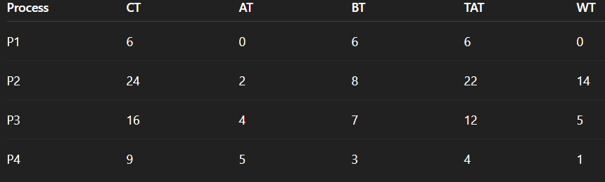
Summary Metrics

• Average Turnaround Time (TAT) = (6 + 22 + 12 + 4)/4 = 1
• Average Waiting Time (WT) = (0 + 14 + 5 + 1)/4 = 5

Algorithms No:04:

Round Robin (RR) Scheduling in Operating Systems

Introduction

Round Robin (RR) is a popular CPU scheduling algorithm widely used in modern operating systems. It is particularly effective for time-sharing systems, where multiple processes or users need to share the CPU fairly.

Round Robin Scheduling Mechanism:

• Each process is assigned a fixed time slice called Time Quantum (TQ).
• When a process’s time quantum expires, the CPU switches to the next process in the ready queue.
• This mechanism ensures fairness, responsiveness, and preemption.

Why Round Robin is Effective

• Fair Scheduling: All processes get a chance to run in cyclic order.
• Best for Multitasking: Ideal for environments with multiple active users or processes.
• Responsive System: Processes don’t have to wait too long, improving overall user experience.

Understanding Time Quantum in Round Robin Scheduling:

Definition

Time Quantum (TQ) is the maximum duration a process can run on the CPU before it is preempted and the CPU switches to the next process in the ready queue.

Examples of Time Quantum

• TQ = 2 ms: Each process runs for a maximum of 2 milliseconds before switching.
• TQ = 5 ms: Each process runs for 5 milliseconds before a context switch occurs.

Choosing the Right Time Quantum

• Good Time Quantum: Small enough to ensure fairness and responsiveness, but not too small to cause excessive context switching.
• Bad Time Quantum: Too large → behaves like FCFS, less responsive. Too small → frequent context switches, high overhead.

Round Robin Scheduling Example (4 Processes)

Criteria: Time Quantum (TQ) = 3 units Mode: Preemptive

Execution Order (Round Robin, TQ=3)

• t=0 → P1 runs for 3 units → remaining BT = 2
• t=3 → P2 runs for 3 units → remaining BT = 0 (finished)
• t=6 → P3 runs for 3 units → remaining BT = 5
• t=9 → P4 runs for 3 units → remaining BT = 3
• t=12 → P1 resumes → runs 2 units → finished
• t=14 → P3 resumes → runs 3 units → remaining BT = 2
• t=17 → P4 resumes → runs 3 units → finished
• t=20 → P3 resumes → runs 2 units → finished

Gantt Chart:

Completion Time (CT):

Turnaround Time (TAT = CT−AT) & Waiting Time (WT = TAT−BT):

Summary Metrics

• Average Turnaround Time (TAT) = (14 + 5 + 18 + 14)/4 = 12.75
• Average Waiting Time (WT) = (9 + 2 + 10 + 8)/4 = 7.25
• CPU Utilization = 100% (No idle time)

Algorithm : No:05

Priority Scheduling in Operating Systems: Complete Guide with Examples

Overview: Priority Scheduling is a CPU scheduling algorithm where each process is assigned a priority number, and the CPU is allocated to the highest priority process. It is widely used in real-time systems, embedded systems, and critical task environments.

In this article, we will cover:

• How Priority Scheduling works
• Types of Priority Scheduling
• Important terms and formulas
• Examples with Gantt Charts
• Step-by-step calculations of CT, TAT, and WT

.What is Priority Scheduling?

Priority Scheduling assigns each process a priority level. The CPU is given to the process with the highest priority first.

Priority Conventions:

• Lower number = higher priority (used in this article)
• Example: Priority 1 > Priority 2 > Priority 3
• Some systems use higher number = higher priority
• Example: Priority 10 > Priority

2. Types of Priority Scheduling

a) Preemptive Priority Scheduling

• If a new process arrives with higher priority, it immediately preempts the currently running process.

b) Non-Preemptive Priority Scheduling

• Once a process gets the CPU, it runs until completion, even if a higher priority process arrives.

Important Terms:

Why Keep TAT & WT Low?

• Low WT → better responsiveness
• Low TAT → faster completion
• Overall Efficiency → better CPU and OS performance

Preemptive Priority Scheduling Example (5 Processes)

Criteria: Lower number = higher priority Mode: Preemptive

Determine Execution Order (Preemptive)

• t=0 → P1 runs (only process)
• t=2 → P2 arrives (Priority 1 < P1 priority 3) → preempt P1, CPU runs P2
• t=4 → P3 arrives (Priority 4 > P2 priority 1) → continue P2
• t=6 → P5 arrives (Priority 5 > P2 priority 1) → continue P2
• t=6 → P2 finishes (BT=4) → choose highest priority in ready queue → P4 (Priority 2)
• t=10 → P4 runs 1 unit, next? P1 remaining=5, P3 arrived=1 → choose P3 (Priority 4)? No, P1 priority 3 > P3 4 → P1? Actually we always pick highest priority → P1 (Priority 3)
• Step-by-step, final Gantt Chart constructed below.

Explanation:

• t=0–2 → P1 runs (remaining 5)
• t=2–6 → P2 (BT=4)
• t=6–10 → P4 (BT=4)
• t=10–13 → P1 resumes (remaining 5 → 2 done)
• t=13–14 → P3 (BT=1)
• t=14–16 → P5 (BT=2)
• t=16–19 → P1 completes remaining 3

Completion Time (CT):

Turnaround Time (TAT = CT−AT) & Waiting Time (WT = TAT−BT):

Summary Metrics:

• Average Turnaround Time (TAT) = (19+4+10+5+10)/5 = 9.6
• Average Waiting Time (WT) = (12+0+9+1+8)/5 = 6
• CPU Utilization = 100% (No idle time)

Non-Preemptive Priority Scheduling Example (5 Processes)

Criteria: Lower number = higher priority Mode: Non-Preemptive

Determine Execution Order

• At t=0 → P1 is only process → CPU runs P1
• t=6 → Processes P2, P3, P4, P5 have arrived → pick highest priority (lowest number) → P2 (Priority 1)
• Next → P4 (Priority 2)
• Then → P1 already finished, next highest priority = P3 (Priority 4)
• Last → P5 (Priority 5)

Gannt Chart:

Completion Time (CT):

Turnaround Time (TAT = CT−AT) & Waiting Time (WT = TAT−BT):

Summary Metrics:

• Average Turnaround Time (TAT) = (6 + 13 + 14 + 22 + 24) / 5 = 15.8
• Average Waiting Time (WT) = (0 + 5 + 11 + 15 + 20) / 5 = 10.2
• CPU Utilization = 100% (No idle time)

Advantages of Priority Scheduling

• Ideal for Real-Time Systems: Handles time-critical tasks efficiently.
• Faster Execution for Important Tasks: High-priority processes complete sooner.
• Flexible Priority Assignment: Allows setting priorities based on task importance.
• Improves Resource Management: Ensures critical tasks get CPU when needed.

Disadvantages of Priority Scheduling

• Starvation: Low-priority processes may wait indefinitely if higher priority tasks keep arriving.
• Indefinite Blocking: Some processes might never get CPU if always out-prioritized.
• Priority Inversion: A lower-priority process may hold a resource needed by a higher-priority process, causing delays.

Solutions to Starvation in Priority Scheduling

Aging Technique:

• Gradually increase the priority of processes that have been waiting for a long time.
• Prevents indefinite waiting for low-priority tasks.
• Ensures fair CPU allocation over time.

Ideal Scenarios for Using Priority Scheduling

1. Real-Time Systems

• Tasks that are time-critical get immediate CPU access.

2. Operating System Kernels

• System processes with different levels of importance are managed efficiently.

3. Embedded Devices

• Devices with multiple tasks of varying urgency prioritize critical operations.

4. Print Queues

• Important or urgent print jobs are completed first.

5. Multimedia Streaming

• Ensures smooth playback by prioritizing time-sensitive processes.

Algorithms No:06:

Multiple-Level Queue (MLQ) Scheduling in Operating Systems

Introduction

Multiple-Level Queue (MLQ) Scheduling is an advanced CPU scheduling method where processes are grouped into different queues based on their priority, type, or class.

Key Features

• Each queue can use a different scheduling algorithm (e.g., FCFS for one queue, Round Robin for another).
• CPU is allocated based on queue priority, ensuring higher-priority queues are served first.
• Processes in higher-priority queues execute before lower-priority queues.
• MLQ is commonly applied in interactive systems and multilevel task management where tasks have varying importance and urgency.

Key Concepts of Multiple-Level Queue (MLQ) Scheduling

1. Multiple Queues

• Processes are divided into separate queues based on priority, type, or importance.

Example:

• Queue 1 → System Processes
• Queue 2 → Interactive Processes
• Queue 3 → Batch Processes

2. Queue Scheduling

• Each queue can implement its own scheduling algorithm, like FCFS or Round Robin.
• CPU allocation among queues is generally priority-based, meaning higher-priority queues are served first.

3. Preemption

• Processes in higher-priority queues can preempt processes in lower-priority queues.
• Ensures that critical tasks get CPU time before less important tasks.Classify Processes: Place all processes into queues according to their type or priority.

How Multiple-Level Queue (MLQ) Scheduling Works:

Assign Scheduling Algorithm: Each queue is assigned a suitable scheduling method (e.g., FCFS, RR).

1. Execute CPU for Highest-Priority Queue: The CPU always executes the highest-priority non-empty queue first.
2. Serve Lower-Priority Queues: Lower-priority queues receive CPU only when higher-priority queues are empty.

Example of Multiple-Level Queue (MLQ) Scheduling

Criteria:

• Queue 1 (High Priority) → System Processes → FCFS
• Queue 2 (Medium Priority) → Interactive Processes → Round Robin (TQ=3)
• Queue 3 (Low Priority) → Batch Processes → FCFS

Execution Order

• Queue 1 (Highest Priority): P1 → P5
• Queue 2 (Medium Priority): P2 → P3 (Round Robin, TQ=3)
• Queue 3 (Lowest Priority): P4

CPU always serves the highest-priority non-empty queue first.

Gantt Chart:

Explanation:

1. t=0–5 → P1 (Queue 1, FCFS)
2. t=5–8 → P5 (Queue 1, FCFS)
3. t=8–11 → P2 (Queue 2, RR, TQ=3)
4. t=11–14 → P3 (Queue 2, RR, TQ=3)
5. t=14–17 → P2 remaining → finished
6. t=17–20 → P3 remaining → finished
7. t=20–28 → P4 (Queue 3, FCFS)

Completion Time (CT):

Turnaround Time (TAT = CT−AT) & Waiting Time (WT = TAT−BT):

Summary Metrics

• Average Turnaround Time (TAT) = (5 + 4 + 13 + 18 + 25)/5 = 13
• Average Waiting Time (WT) = (0 + 1 + 9 + 12 + 17)/5 = 7.8
• CPU Utilization = 100% (No idle time)

Advantages of Multiple-Level Queue (MLQ) Scheduling

• Handles Different Types of Processes: Works well for system, interactive, and batch processes.
• Efficient CPU Usage: Ensures CPU is utilized effectively in environments with multiple process types.
• Flexible Scheduling: Each queue can use a different scheduling algorithm suited to its process type.
• Reduces Starvation (with Aging): Low-priority processes are eventually executed if aging technique is applied.

Disadvantages of Multiple-Level Queue (MLQ) Scheduling

• Complex Implementation: More difficult to implement compared to simple scheduling methods like FCFS or RR.
• Starvation Risk: Processes in lower-priority queues may have to wait a long time if higher-priority queues are always full.
• Choosing Correct Settings is Tricky: Assigning queue priorities and scheduling algorithms for each queue can be challenging.
• Needs Careful Tuning: Real-world systems require fine-tuning to ensure balanced performance.

Real-Life Applications of Multiple-Level Queue (MLQ) Scheduling

1. Operating System Kernels

• Used to manage system processes efficiently, giving higher priority to critical tasks.

2. Multi-User Systems

• Handles interactive and batch jobs fairly, ensuring important tasks don’t wait too long.

3. Multimedia Systems

• Prioritizes high-priority video or audio tasks to maintain smooth playback.

4. Cloud Computing Environments

• Manages different types of workloads with varying priorities in virtual machines and servers.

5. Time-Sharing Systems

• Ensures fair CPU access for all users while giving preference to more critical tasks.

FAQ — Multiple-Level Queue (MLQ) Scheduling

1. How is MLQ different from Multilevel Feedback Queue (MLFQ)?

• MLQ: Each process stays permanently in its assigned queue.
• MLFQ: Processes can move between queues based on their behavior or CPU usage.

2. Can each queue use a different scheduling algorithm?

• Yes. For example, one queue can use FCFS while another uses Round Robin (RR) depending on the type of process.

3. How is starvation prevented?

• By applying aging, which gradually increases the priority of waiting processes.
• Some CPU time can be reserved for lower-priority queues to ensure fairness.

4. Is MLQ preemptive?

• Yes. Processes in higher-priority queues can preempt those in lower-priority queues.