Naive Bayes in Detail Explanation

In this article we will learn Probability-based Classification technique called Naive Bayes.

In this blog we will be covering below topics -

1. What is Naive Bayes?
2. Math behind Naive Bayes algorithm
3. Naive Bayes with example
4. Naive Bayes On text-data and Laplace smoothing
5. Naive Bayes for large dimensionality data
6. Bais-variance tradeoff, Feature Importance and Interpretation of Naive Bayes
7. Types of Naive Bayes Classifiers
8. Pros and Cons of Naive Bayes
9. Applications of Naive Bayes Algorithm

1. What is Naive Bayes?

Naive Bayes is a probabilistic algorithm used in machine learning for classification problems. It is based on Bayes’ theorem, which states that the probability of an event occurring given prior knowledge about related events can be calculated using conditional probability.

Naive Bayes is “naive” because it assumes that the features of a data point are independent of each other. This is often not true in real-world data, but the assumption simplifies the calculations and can still provide good results in practice.

Bayes theorem :

Bayes’ Theorem describes the probability of an event, based on a prior knowledge of conditions that might be related to that event.

What makes Naive Bayes a “Naive” algorithm?

Naive Bayes classifier assumes that the features we use to predict the target are independent and do not affect each other. While in real-life data, features depend on each other in determining the target, but this is ignored by the Naive Bayes classifier.

Though the independence assumption is never correct in real-world data, but often works well in practice. so that it is called “Naive”.

2. Math behind Naive Bayes Algorithm

Given a features vector X=(x1,x2,…,xn) and a class variable y, Bayes Theorem states that:

We’re interested in calculating the posterior probability P(y | X) from the likelihood P(X | y) and prior probabilities P(y),P(X).

Using the chain rule, the likelihood P(X ∣ y) can be decomposed as:

but because of the Naive’s conditional independence assumption, the conditional probabilities are independent of each other.

Thus, by conditional independence, we have:

And as denominator remains constant for all values, the posterior probability can then be:

The Naive Bayes classifier combines this model with a decision rule. One common rule is to pick the hypothesis that’s most probable; this is known as the maximum a posteriori or MAP decision rule.

3. Naive Bayes with example:

Let’s explain it using an example to make things clear:

Consider a fictional dataset that describes the weather conditions for playing a game of golf. Given the weather conditions, each tuple classifies the conditions as fit(“Yes”) or unfit(“No”) for playing golf.

Here is a tabular representation of our dataset.

The dataset is divided into two parts, namely, feature matrix and the response vector.

• Feature matrix contains all the vectors(rows) of dataset in which each vector consists of the value of dependent features. In above dataset, features are ‘Outlook’, ‘Temperature’, ‘Humidity’ and ‘Windy’.
• Response vector contains the value of class variable(prediction or output) for each row of feature matrix. In above dataset, the class variable name is ‘Play golf’.

Learning phase:

In the learning phase we need to compute the table of likelihoods from the training data,

we need to find ,

(1) P(outlook = O / Play Golf=b);

where O ∈ {Sunny, Overcast, Rainy}, b ∈ {yes, no}

(2) P(temperature = t / Play Golf=b);

where t ∈ {Hot, Mild, Cool}

(3) P(Humidity = h / Play Golf=b);

where h ∈ {high, normal}

(4) P(windy = w / Play Golf=b);

where w ∈ {True, False}

Classification phase:

If we get new instance,

x’ = (Outlook = sunny, temperature = Cool, Humidity = High, wind = True)

what is class of x’?

So, probability of playing golf is given by:

P(Play Golf = yes / x’)

= ( P(Outlook = sunny/Play Golf = yes) P(temperature = Cool/Play Golf = yes) P(Humidity = High/Play Golf = yes) P(Wind = True/Play Golf = yes) P(Play Golf = yes) ) / P(x’)

probability to not play golf is given by:

P(Play Golf = No/ x’)

= ( P(Outlook = sunny/Play Golf = No) P(temperature = Cool/Play Golf = No) P(Humidity = High/Play Golf = No) P(Wind = True/Play Golf = No) P(Play Golf = No) ) / P(x’)

Since, denominator P(x’) is common in both probabilities, we can ignore P(x’) and find proportional probabilities as:

So, probability of playing golf is:

P(Play Golf = yes / x’)

= ( P(Outlook = sunny/Play Golf = yes) P(temperature = Cool/Play Golf = yes) P(Humidity = High/Play Golf = yes) P(Wind = True/Play Golf = yes) P(Play Golf = yes) )

= (2/9)(3/9)(3/9)(3/9)(9/14)

=0.0053

probability to not play golf is:

P(Play Golf = No/ x’)

= ( P(Outlook = sunny/Play Golf = No) P(temperature = Cool/Play Golf = No) P(Humidity = High/Play Golf = No) P(Wind = True/Play Golf = No) P(Play Golf = No) )

= (3/5)(1/5)(4/5)(3/5)(5/14)

=0.0205

here P(Play Golf = No/ x’) > P(Play Golf = yes/ x’)

So, prediction that golf would be played is ‘No’.

we have seen Naive Bayes work well on Catagorical Data,

Now we will see Naive Bayes on text-data.

4. Naive Bayes On text-data and Laplace smoothing:

4.1 Naive Bayes On text-data :

Naive bayes work well on text-data,

for example spam filter(email : spam/not spam), review(+ve/-ve) are the applications of Naive Bayes.

for example we have review data like this,

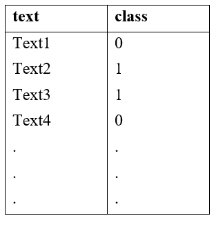
our task is to predict whether the review is +ve/-ve.

Task : compare P(y=1/text(i)) and P(y=0/text(i)) for given text(i) , Whichever is higher we decide that class as a class of given text(i).

first of all we have to complete all the preprocessing steps of text-data, like remove stop-words, stemming, n-grams. after apply all those step we get bunch of words, then we compute binary bag of words.

now , we have text → {w1,w2,w3….wd}

so, P(y=1/text(i)) = P(y=1/w1,w2,w3…wd) ∝ P(y=1)P(w1/y=1)P(w2/y=1)…..P(wd/y=1)

same for P(y=0/text(i)) =P(y=0/w1,w2,w3…wd) ∝ P(y=0)P(w1/y=0)P(w2/y=0)…..P(wd/y=0)

we can compute, P(wi/y=0) = (no. of data points which contain wi and y=0)/(no. of data points with y=0)

P(wi/y=1) = (no. of data points which contain wi and y=1)/(no. of data points with y=1)

In this way we can apply Naive Bayes on text-data.

Note : In text-classification problems Naive Bayes is a very good baseline. so for text-classification problem Naive Bayes is on benchmark compare to other algorithms.

problem :

Let’s take an example of text classification where the task is to classify whether the review Is positive or negative. We build a likelihood table based on the training data. While querying a review, we use the Likelihood table values, but what if a word in a review was not present in the training dataset?

Query review = w1 w2 w3 w’

We have four words in our query review, and let’s assume only w1, w2, and w3 are present in training data. So, we will have a likelihood for those words. To calculate whether the review is positive or negative, we compare P(positive|review) and P(negative|review).

In the likelihood table, we have P(w1|positive), P(w2|Positive), P(w3|Positive), and P(positive). Oh, wait, but where is P(w’|positive)?

If the word is absent in the training dataset, then we don’t have its likelihood. What should we do?

Approach1- Ignore the term P(w’|positive)

Ignoring means that we are assigning it a value of 1, which means the probability of w’ occurring in positive P(w’|positive) and negative review P(w’|negative) is 1. This approach seems logically incorrect.

Approach 2- In a bag of words model, we count the occurrence of words. The occurrences of word w’ in training are 0. According to that

P(w’|positive)=0 and P(w’|negative)=0, but this will make both P(positive|review) and P(negative|review) equal to 0 since we multiply all the likelihoods. This is the problem of zero probability. So, how to deal with this problem?

4.2 Laplace Smoothing :

Laplace smoothing is a smoothing technique that handles the problem of zero probability in Naïve Bayes. Using Laplace smoothing, we can represent P(w’|positive) as

Here, alpha represents the smoothing parameter, K represents the number of dimensions (features) in the data, and N represents the number of reviews with y=positive

If we choose a value of alpha!=0 (not equal to 0), the probability will no longer be zero even if a word is not present in the training dataset.

Interpretation of changing alpha

Let’s say the occurrence of word w is 3 with y=positive in training data. Assuming we have 2 features in our dataset, i.e., K=2 and N=100 (total number of positive reviews).

Case 1- when alpha=1

P(w’|positive) = 3/102

Case 2- when alpha = 100

P(w’|positive) = 103/300

Case 3- when alpha=1000

P(w’|positive) = 1003/2100

As alpha increases, the likelihood probability moves towards uniform distribution (0.5). Most of the time, alpha = 1 is being used to remove the problem of zero probability.

In short, Laplace smoothing is a smoothing technique that helps tackle the problem of zero probability in the Naïve Bayes machine learning algorithm. Using higher alpha values will push the likelihood towards a value of 0.5, i.e., the probability of a word equal to 0.5 for both the positive and negative reviews. Since we are not getting much information from that, it is not preferable. Therefore, it is preferred to use alpha=1.

5. Naive Bayes for large dimensionality data :

Naive Bayes work well on text-data with high dimension, but we have to use log-probability for numerical stability.

Read more about log-probability here.

6. Bais-variance tradeoff, Feature Importance and Interpretation of Naive Bayes :

6.1 Bias-variance tradeoff :

In Naive Bayes, α (hyper parameter) of laplace smoothing determine underfitting and overfitting.

small α → high varience → Overfitting

large α → high bias → underfitting

so, choose right α using simple cross-validation/k-fold CV.

6.2 Feature Importance :

In many algorithms like KNN we have to compute feature Importance Using forward feature selection or other techniques, But in Naive Bayes gives feature Importance determine/obtain directly from the model.

for +ve class : find words(wi) with highest value of P(wi/y=1) for -ve class : find words(wi) with highest value of P(wi/y=0)

both are obtain from the model

1. sort all wi’s based on P(wi/y=1) in desc order, wi’s with high value of P(wi/y=1) → Important words/features in determining that data point ∈ +ve class.
2. sort all wi’s based on P(wi/y=0) in desc order, wi’s with high value of P(wi/y=0) → Important words/features in determining that data point ∈ -ve class.

6.3 Interpretation :

In Naive Bayes we can easily Interprete our model using likelihood/probability.

7. Types of Naive Bayes Classifiers :

• Multinomial: Feature vectors represent the frequencies with which certain events have been generated by a multinomial distribution. For example, the count how often each word occurs in the document. This is the event model typically used for document classification.
• Bernoulli: Like the multinomial model, this model is popular for document classification tasks, where binary term occurrence(i.e. a word occurs in a document or not) features are used rather than term frequencies(i.e. frequency of a word in the document).
• Gaussian: It is used in classification and it assumes that features follow a normal distribution.

8. Pros and Cons of Naive Bayes :

Pros:

1. In text-classification Naive bayes is a baseline/benchmark.
2. Naive Bayes is Interpretable and give feature importance.
3. Run-time and Train-time complexity is low, run time space is also low.
4. When the Naive Bayes conditional independence assumption holds true, it will converge quicker than discriminative models like logistic regression.

Cons:

1. The assumption of independent predictors/features. Naive Bayes implicitly assumes that all the attributes are mutually independent which is almost impossible to find in real-world data.
2. In text-data Naive Bayes can easily overfit if we don’t do laplace smoothing, choose right α using cross-validation.
3. Naive Bayes work well for categorical features, but for real-value features Naive Bayes can’t use much.

9. Applications of Naive Bayes Algorithm :

• Real-time Prediction.
• Text classification/ Spam Filtering/ Sentiment Analysis.
• Language Detection etc.

Thanks for reading!

please! Don’t forget to clap if You have understand topic clearly

Please write comments if you find anything incorrect, or you want to share more information about the topic discussed above.