How to Create a Digital “Data-Mode” Contour Animation in Processing
Generative art has a way of turning simple math into something strangely alive. In this tutorial, we’ll build a hypnotic “data-mode”…
How to Create a Digital “Data-Mode” Contour Animation in Processing
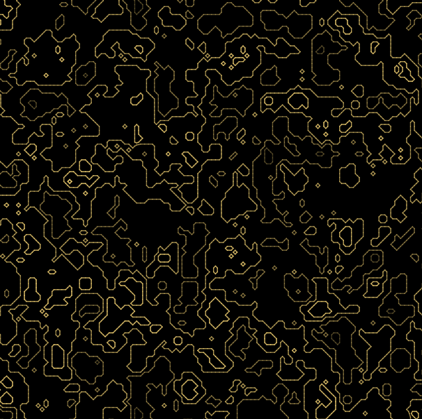
Generative art has a way of turning simple math into something strangely alive. In this tutorial, we’ll build a hypnotic “data-mode” contour animation — like watching a topographic scan flicker across a futuristic display.
Using nothing more than Processing 4.3.2, Perlin noise, and a classic algorithm called Marching Squares, we’ll create:
✔ A living digital terrain ✔ Quantized “data slice” aesthetics ✔ Smooth, seamless looping ✔ And a direct GIF export
Everything runs in Java mode with one small library, and the results look like they came straight out of a sci-fi UI panel.
🚀 Overview
We’ll build this animation in five main steps:
- Create a noise field
- Quantize it into digital steps
- Use Marching Squares to generate contour lines
- Animate the field over time
- Export the animation as a GIF
By the end, you’ll have a fully functional Processing sketch that produces this hypnotic effect:
A pulsing, glowing, animated digital topography built entirely from math.
📦 Requirements
You’ll need:
- Processing 4.3.2 (Java mode)
- GifAnimation library Install via:
Sketch → Import Library → Add Library → Search “GifAnimation” → Install
That’s it.
🧠 How It Works
Before we dive into the code, let’s break down the three ideas that make this animation possible.
1. Perlin Noise → A Smooth Height Map
Processing’s noise() function gives us a natural, organic texture.
We sample it across a grid and store the values in a 2D array called field.
This becomes our digital “height map.”
2. Quantization → Digital Slices
Instead of using the raw smooth noise, we snap values into discrete levels:
0.0
0.2
0.4
0.6
0.8
1.0
These slices feel like:
- medical imaging
- sonar scans
- elevation data
- glitchy machine-vision layers
This is the “data mode” aesthetic.
3. Marching Squares → Contour Lines
Marching Squares is an algorithm that:
- looks at four corners of a tiny square
- checks which corners are above a threshold
- draws a line segment where the field crosses that threshold
We run Marching Squares for several thresholds (“iso-values”) to build layered contour lines.
The magic is that every tiny segment aligns perfectly with its neighbors, producing smooth, continuous curves.
🧾 Full Working Code (Ready to Run)
Create a new empty sketch in Processing and paste this entire code:
// Quantized "Data Mode" Noise Contour Field — WITH GIF EXPORT
// Processing 4.3.2 (Java Mode)
// Press 'g' to export a seamless looping GIF
import gifAnimation.*;int W = 540;
int H = 960;float cellSize = 10;
int cols, rows;float[][] field;float noiseScale = 0.015;
float radius = 2.0;
int loopFrames = 240; // frames per full seamless loopint quantLevels = 6; // discrete noise stepsGifMaker gif;
boolean exporting = false;
int gifFrame = 0;void setup() {
size(W, H); // safest in Processing 4.3.2 cols = int(W / cellSize) + 2;
rows = int(H / cellSize) + 2;
field = new float[cols][rows]; smooth(8);
colorMode(RGB, 255);
strokeCap(ROUND);
noFill();
}void draw() {
background(0); // time variable (looping)
float u = exporting ? gifFrame / float(loopFrames)
: (frameCount % loopFrames) / float(loopFrames); float angle = TWO_PI * u;
float nzx = cos(angle) * radius;
float nzy = sin(angle) * radius; // ---- quantized noise sampling ----
for (int j = 0; j < rows; j++) {
for (int i = 0; i < cols; i++) {
float x = i * cellSize;
float y = j * cellSize; float n = noise(x * noiseScale + nzx, y * noiseScale + nzy);
float q = floor(n * quantLevels); // quantize
q = q / (quantLevels - 1.0); // normalize to 0..1 field[i][j] = q;
}
} // ---- draw contours between levels ----
int levels = quantLevels - 1;
for (int k = 0; k < levels; k++) {
float iso = (k + 0.5) / (quantLevels - 1.0); float alpha = map(k, 0, levels - 1, 60, 220);
stroke(255, 220, 120, alpha);
strokeWeight(1.8); marchingSquares(iso);
} // ---- GIF capture ----
if (exporting) {
gif.addFrame();
gifFrame++; if (gifFrame >= loopFrames) {
gif.finish();
exporting = false;
println("GIF export completed ✔ Saved as export.gif");
}
}
}// marching squares
void marchingSquares(float iso) {
for (int j = 0; j < rows - 1; j++) {
for (int i = 0; i < cols - 1; i++) { float a = field[i][j];
float b = field[i+1][j];
float c = field[i+1][j+1];
float d = field[i][j+1]; int state = 0;
if (a > iso) state |= 1;
if (b > iso) state |= 2;
if (c > iso) state |= 4;
if (d > iso) state |= 8; if (state == 0 || state == 15) continue; PVector pA = new PVector(i * cellSize, j * cellSize);
PVector pB = new PVector((i+1)*cellSize, j * cellSize);
PVector pC = new PVector((i+1)*cellSize, (j+1)*cellSize);
PVector pD = new PVector(i * cellSize, (j+1)*cellSize); PVector p0 = interp(pA, pB, a, b, iso);
PVector p1 = interp(pB, pC, b, c, iso);
PVector p2 = interp(pC, pD, c, d, iso);
PVector p3 = interp(pD, pA, d, a, iso); switch (state) {
case 1: drawSeg(p3, p0); break;
case 2: drawSeg(p0, p1); break;
case 3: drawSeg(p3, p1); break;
case 4: drawSeg(p1, p2); break;
case 5: drawSeg(p3, p0); drawSeg(p1, p2); break;
case 6: drawSeg(p0, p2); break;
case 7: drawSeg(p3, p2); break;
case 8: drawSeg(p2, p3); break;
case 9: drawSeg(p0, p2); break;
case 10: drawSeg(p0, p1); drawSeg(p2, p3); break;
case 11: drawSeg(p1, p2); break;
case 12: drawSeg(p3, p1); break;
case 13: drawSeg(p0, p1); break;
case 14: drawSeg(p3, p0); break;
}
}
}
}PVector interp(PVector p1, PVector p2, float v1, float v2, float iso) {
float denom = (v2 - v1);
float t = (abs(denom) < 1e-6) ? 0.5 : (iso - v1) / denom;
return PVector.lerp(p1, p2, constrain(t, 0, 1));
}// draw line segment
void drawSeg(PVector a, PVector b) {
beginShape();
vertex(a.x, a.y);
vertex(b.x, b.y);
endShape();
}// ---------- press 'g' to export ----------
void keyPressed() {
if (key == 'g' || key == 'G') {
println("Starting GIF export...");
exporting = true;
gifFrame = 0;
gif = new GifMaker(this, "export.gif");
gif.setRepeat(0); // loop forever
gif.setQuality(10);
gif.setDelay(1000/60); // ~60 FPS
}
}🔍 How the Contour Lines Are Actually Made
If you’re curious how the animation generates those silky contour lines, here’s the breakdown.
🔸 Step 1 — Build a 2D height map
We store quantized noise values in a grid:
field[i][j] = q;Each value is a discrete “height” from 0 to 1.
🔸 Step 2 — Choose iso-values (the boundaries)
To create a contour, we pick a threshold:
float iso = 0.3;The contour line is drawn everywhere that the field crosses this value.
🔸 Step 3 — Look at a 2×2 block of the grid
Each block has four corners:
a ---- b
|      |
d ---- c
We ask:
Which corners are above the iso level?
This gives a 4-bit “state” between 0 and 15.
🔸 Step 4 — Marching Squares connects the dots
Depending on the state, the contour crosses certain edges.
We compute the exact crossing point with interpolation:
PVector p0 = interp(pA, pB, a, b, iso);Then we draw a small segment between two edges.
Do this across the entire grid, and the segments merge into smooth curves.
That’s it. That’s how the map is drawn.
🎬 Exporting a Seamless GIF
Once the animation is running:
- Press G
- Processing records one full loop
- When finished, you’ll see:
GIF export completed ✔ Saved as export.gifThe GIF is ready to post anywhere.
Variations to Explore
Once you understand the core idea, try modifying:
✔ quantLevels
More levels → more contour lines Fewer levels → big graphic shapes
✔ Color palette
Change RGB values for neon, cyan, magenta, amber, grayscale…
✔ Swirl or warp the coordinates
Add rotation based on distance from center for vortex effects.
✔ Add glow
Switch to P2D + blendMode(ADD) (some systems only).
🎉 Final Thoughts
These kinds of generative animations let you explore the boundary between math and aesthetics. A simple noise field combined with contour extraction can look like:
- magnetic fields
- alien terrain
- medical imaging
- glitchy machine vision
The power comes from layering the simplest ideas possible.
If you create something cool with this, definitely share it — the variations are endless.
메타데이터
- post_id
- c3ebc98cd34d
- slug
- how-to-create-a-digital-data-mode-contour-animation-in-processing-c3ebc98cd34d
- url
- https://medium.com/@rh.h.rad/how-to-create-a-digital-data-mode-contour-animation-in-processing-c3ebc98cd34d
- canonical_url
- https://medium.com/@rh.h.rad/how-to-create-a-digital-data-mode-contour-animation-in-processing-c3ebc98cd34d
- author_url
- https://medium.com/@rh.h.rad
- status
- ok
- fetched_at
- 2026-06-26 21:52:29