Efficiently Utilizing Your GPU While Training AI Models in PyTorch

A practical, code-first guide to making your training loop go at a lightning speed without rewriting everything from scratch.

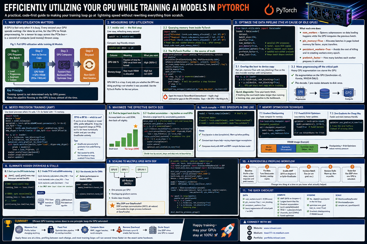
Fig 1: Efficiently Utilizing Your GPU While Training AI Models in PyTorch

Table of Contents

1. Why GPU Utilization Matters

2. Measuring GPU Utilization

2.1 nvidia-smi — The First Stop

2.2 Querying Memory from Inside PyTorch

2.3 The PyTorch Profiler — The Source of Truth

3. Optimize the Data Pipeline — The #1 Cause of Idle GPUs

3.1 Overlap the Host toDevice Copy

3.2 Move Preprocessing Off the Critical Path

4. Mixed Precision Training (AMP)

5. Maximize the Effective Batch Size

5.1 Find the Largest Batch That Fits

5.2 Gradient Accumulation — Big Batches on Small GPUs

6. torch.compile — Free Speedups in One Line

7. Memory Optimization Techniques

7.1 Gradient (Activation) Checkpointing

7.2 Fused and Memory-Efficient Optimizers

7.3 Zero Gradients the Cheap Way

8. Eliminate Hidden Overhead and Stalls

8.1 Don’t Synchronize the GPU Inside the Training Loop

8.2 Enable TF32 and cuDNN Autotuning

8.3 Use channels_last for CNNs

9. Scaling to Multiple GPUs with Distributed Data Parallel (DDP)

10. A Reproducible Profiling Workflow

11. The Quick Checklist

12. Summary

1. Why GPU Utilization Matters

A GPU is fast only when it is busy. Every second your GPU spends waiting — for data to arrive, for the CPU to finish preprocessing, for a tensor to copy across the PCIe bus — is a second of compute (and money) thrown away.

Fig 2: Full GPU utilization while training AI Models

The mental model is simple:

Fig: 1 illustrates the high-level training pipeline used in deep learning systems and shows how the CPU and GPU collaborate during model training. At a high level, the workflow follows a continuous loop:

Step 1: CPU Prepares the Batch

The CPU is responsible for handling the input pipeline before computation begins. This includes:

Loading samples from disk

Applying preprocessing or augmentations

Tokenization or image transformations

Collating samples into batches

In PyTorch, this stage is usually handled by the DataLoader and worker processes. If the CPU is too slow at preparing batches, the GPU becomes idle while waiting for data, reducing overall utilization.

Step 2: Host to Device Copy

Once a batch is ready, it is copied from:

Host memory (CPU RAM) to Device memory (GPU VRAM)

This transfer typically happens over:

PCIe

NVLink (on high-end systems)

Data transfer can become a bottleneck if:

batches are too small,

memory is not pinned,

preprocessing is slow,

or transfers are synchronous.

Efficient pipelines try to overlap data transfer with GPU computation so the GPU never waits for the next batch.

Step 3: GPU Computes

After the batch reaches GPU memory, the GPU performs the actual deep learning computation:

Forward pass

Loss computation

Backward pass (gradient calculation)

Optimizer update

This is where matrix multiplications and tensor operations happen in parallel across thousands of GPU cores. High GPU utilization means the GPU spends most of its time executing these operations rather than waiting for data.

Step 4: Repeat

After one batch finishes:

The next batch is prepared on the CPU

Copied to the GPU

Computed on by the GPU

This loop repeats at every training iteration. The goal of performance optimization is to keep this pipeline flowing continuously with minimal idle time.

Why This Figure Matters

The figure highlights an important principle in deep learning systems:

Training speed is not determined only by GPU power.

Even with a powerful GPU, poor data loading, slow preprocessing, inefficient memory transfer, or synchronization stalls can leave the GPU underutilized.

A well-optimized training pipeline ensures:

The CPU prepares data fast enough

Transfers overlap with computation

The GPU remains busy almost all the time

This is what people mean by full GPU utilization.

If any step in that chain is slower than the GPU compute itself, the GPU sits idle. Your job is to make the GPU the bottleneck — because if the most expensive component is the busiest one, you’re using your hardware efficiently.

The golden rule: You can’t optimize what you can’t measure. Always profile before and after a change. Intuition about performance is frequently wrong.

2. Measuring GPU Utilization

Before touching the training loop, learn to read what your GPU is actually doing.

2.1 nvidia-smi — the first stop

Live view, refreshing every second

watch -n 1 nvidia-smi

Fig 3: GPU Utilization Reatime

Compact, log-friendly stream of utilization + memory

nvidia-smi dmon -s um

Look at two numbers in

GPU-Util % is a trap. It only tells you whether the GPU was doing anythingnot whether it was saturated. A tiny kernel running 100% of the time shows 100% util while using 5% of the actual compute. Use the PyTorch Profiler (below) for the real picture.

2.2 Querying memory from inside PyTorch

import torch
print(f"Allocated: {torch.cuda.memory_allocated() / 1e9:.2f} GB")
print(f"Reserved: {torch.cuda.memory_reserved() / 1e9:.2f} GB")
print(f"Peak: {torch.cuda.max_memory_allocated() / 1e9:.2f} GB")
# Reset the peak counter between phases (e.g., after warmup)
torch.cuda.reset_peak_memory_stats()

2.3 The PyTorch Profiler — the source of truth

from torch.profiler import profile, ProfilerActivity, schedule
with profile(
 activities=[ProfilerActivity.CPU, ProfilerActivity.CUDA],
 schedule=schedule(wait=1, warmup=1, active=3, repeat=1),
 on_trace_ready=torch.profiler.tensorboard_trace_handler("./log"),
 record_shapes=True,
 profile_memory=True,
 with_stack=True,
) as prof:
 for step, (x, y) in enumerate(dataloader):
 train_step(x, y)
 prof.step() # tell the profiler a step finished
 if step >= 6:
 break
# Quick text summary, sorted by GPU time
print(prof.key_averages().table(sort_by="cuda_time_total", row_limit=15))

Open the trace in TensorBoard (tensorboard — logdir ./log) and look for gaps on the GPU timeline. Gaps = idle GPU = the thing to fix.

3. Optimize the Data Pipeline (the #1 cause of idle GPUs)

The most common reason a GPU is underutilized is that the **CPU can’t feed it fast enough. PyTorch’s DataLoader has several knobs that solve this.

from torch.utils.data import DataLoader
loader = DataLoader(
 dataset,
 batch_size=256,
 shuffle=True,
 num_workers=8, # parallel CPU processes that build batches
 pin_memory=True, # faster, async host→device transfers
 persistent_workers=True, # don't respawn workers every epoch
 prefetch_factor=4, # batches each worker preloads ahead of time
 drop_last=True, # keeps batch shapes constant (helps compile/cudnn)
)

What each one does:

num_workers — Spawns subprocesses so data loading happens while the GPU computes the previous batch. Start around the number of physical CPU cores and tune from there. Too many can cause contention. pin_memory=True — Allocates batches in page-locked memory, which lets the GPU copy them asynchronously and faster. persistent_workers=True — Avoids the cost of killing and re-creating workers at the start of every epoch. prefetch_factor — How many batches each worker prepares in advance.

3.1 Overlap the host to device copy

Pair pin_memory=True with non_blocking=True so the data transfer overlaps with computation instead of blocking it:

for x, y in loader:
 x = x.to(device, non_blocking=True)
 y = y.to(device, non_blocking=True)
 # … GPU can start the next copy while this batch trains

Quick diagnostic: Wrap your batch-fetch in a timer. If fetching the next batch takes longer than running a training step on it, your pipeline is the bottleneck — fix this before anything else.

3.2 Move preprocessing off the critical path

Heavy CPU augmentation (resizing, decoding) can starve the GPU. Options:

Do augmentation on the GPU (e.g., with torchvision.transforms.v2 on tensors, or libraries like Kornia / NVIDIA DALI). Pre-decode/pre-resize datasets to disk once, instead of every epoch.

4. Mixed Precision Training (AMP)

Modern GPUs (Volta and newer) have Tensor Cores that run half-precision matmuls dramatically faster than FP32. Automatic Mixed Precision (AMP) uses lower precision where it’s safe and keeps FP32 where it matters — typically 1.5–3× faster with roughly half the memory, at little or no accuracy cost.

import torch
device = "cuda"
model = model.to(device)
optimizer = torch.optim.AdamW(model.parameters(), lr=3e-4)
# GradScaler prevents fp16 gradients from underflowing to zero.
# Not needed for bf16, but harmless to keep enabled=False there.
use_fp16 = True
scaler = torch.amp.GradScaler("cuda", enabled=use_fp16)
amp_dtype = torch.float16 if use_fp16 else torch.bfloat16
for x, y in loader:
 x = x.to(device, non_blocking=True)
 y = y.to(device, non_blocking=True)
optimizer.zero_grad(set_to_none=True)
# Run the forward pass in mixed precision
 with torch.autocast(device_type="cuda", dtype=amp_dtype):
 preds = model(x)
 loss = loss_fn(preds, y)
# Scale loss >> backward >> unscale >> step
 scaler.scale(loss).backward()
 scaler.step(optimizer)
 scaler.update()

FP16 vs BF16 — which to use?

Fig 4: FP16 vs BF16 Comparision

If you’re on an Ampere or newer GPU, prefer bfloat16. It has the same exponent range as FP32, so it’s far more numerically stable and you can drop the GradScaler entirely.

5. Maximize the Effective Batch Size

Larger batches give the GPU more work per kernel launch, improving the compute-to-overhead ratio. But you’re limited by VRAM. Two techniques help.

5.1 Find the largest batch that fits

Increase the batch size until you hit an out-of-memory error, then back off slightly. A simple manual sweep or a binary search works well; some frameworks (e.g., PyTorch Lightning’s tuner) automate it.

5.2 Gradient accumulation — big batches on small GPUs

Simulate a large batch by summing gradients over several smaller “micro-batches” before stepping the optimizer:

accum_steps = 4 # effective batch = batch_size * accum_steps
optimizer.zero_grad(set_to_none=True)
for i, (x, y) in enumerate(loader):
 x = x.to(device, non_blocking=True)
 y = y.to(device, non_blocking=True)
with torch.autocast(device_type="cuda", dtype=amp_dtype):
 loss = loss_fn(model(x), y)
 loss = loss / accum_steps # normalize so the sum averages correctly
scaler.scale(loss).backward() # accumulates into .grad
if (i + 1) % accum_steps == 0:
 scaler.step(optimizer)
 scaler.update()
 optimizer.zero_grad(set_to_none=True)

Remember to divide the loss by accum_steps — otherwise your effective learning rate scales up by that factor. Also call optimizer.step() only on accumulation boundaries.

6. torch.compile — Free Speedups in One Line

Since PyTorch 2.0, torch.compile JIT-compiles your model into fused, optimized kernels. It often delivers a 20–50%+ speedup with a single line of code.

model = torch.compile(model) # that's it
# Optional modes:
# model = torch.compile(model, mode="reduce-overhead") # great for small models
# model = torch.compile(model, mode="max-autotune") # slow compile, fast runtime

Practical notes:

The first iteration is slow (it compiles). Warmup before profiling. Constant input shapes help — varying shapes trigger expensive recompilation. Use drop_last=True and fixed sequence lengths where possible. It composes cleanly with AMP and DDP — apply torch.compile to the base model, then wrap with DDP.

7. Memory Optimization Techniques

When you’re VRAM-bound, these let you train bigger models or use bigger batches.

7.1 Gradient (activation) checkpointing

Trade compute for memory: instead of storing all activations for the backward pass, recompute them on the fly. This can cut activation memory massively at the cost of ~20–30% more compute.

from torch.utils.checkpoint import checkpoint_sequential
# For an nn.Sequential of N blocks, checkpoint in `segments` chunks
out = checkpoint_sequential(model.layers, segments=4, input=x, use_reentrant=False)

For custom modules, wrap the expensive forward with torch.utils.checkpoint.checkpoint(fn, args, use_reentrant=False)*.

7.2 Fused and memory-efficient optimizers

# Fused optimizer kernels reduce launch overhead (single kernel for the update)
optimizer = torch.optim.AdamW(model.parameters(), lr=3e-4, fused=True)

For very large models, consider 8-bit optimizers (e.g., bitsandbytes) to shrink optimizer state, which is often the largest memory consumer after activations.

7.3 Zero gradients the cheap way

optimizer.zero_grad(set_to_none=True) # frees the grad buffers instead of writing zeros

set_to_none=True is the default in recent PyTorch and is both faster and more memory-friendly.

8. Eliminate Hidden Overhead and Stalls

These small things quietly destroy throughput.

8.1 Don’t sync the GPU inside the loop

CUDA runs asynchronously. Calling .item(), .cpu(), print(loss), or loss.numpy() every step forces the CPU to wait for the GPU to finish, stalling the pipeline.

#Forces a sync every step
running_loss += loss.item()
# Accumulate on-device, sync occasionally (e.g., once per epoch)
running_loss += loss.detach()
# … later:
print(running_loss.item() / num_steps)

8.2 Enable TF32 and cuDNN autotuning

# TF32: faster matmuls on Ampere+ with negligible accuracy impact
torch.backends.cuda.matmul.allow_tf32 = True
torch.backends.cudnn.allow_tf32 = True
# Let cuDNN benchmark and cache the fastest conv algorithm.
# Use ONLY when input sizes are constant across iterations.
torch.backends.cudnn.benchmark = True

8.3 Use channels_last for CNNs

For convolutional models, the channels_last memory format maps better onto Tensor Cores:

model = model.to(memory_format=torch.channels_last)
x = x.to(memory_format=torch.channels_last)

9. Scaling to Multiple GPUs with DDP

When one GPU isn’t enough, use DistributedDataParallel (DDP) — not the older DataParallel, which is slower and bottlenecks on a single process.

# train.py - launch with: torchrun - nproc_per_node=4 train.py
import os, torch
import torch.distributed as dist
from torch.nn.parallel import DistributedDataParallel as DDP
from torch.utils.data.distributed import DistributedSampler
def main():
 dist.init_process_group(backend="nccl")
 local_rank = int(os.environ["LOCAL_RANK"])
 torch.cuda.set_device(local_rank)
 device = torch.device("cuda", local_rank)
model = MyModel().to(device)
 model = DDP(model, device_ids=[local_rank])
sampler = DistributedSampler(dataset) # splits data across GPUs, no overlap
 loader = DataLoader(dataset, batch_size=256, sampler=sampler,
 num_workers=8, pin_memory=True)
for epoch in range(epochs):
 sampler.set_epoch(epoch) # ensures different shuffling per epoch
 for x, y in loader:
 x, y = x.to(device, non_blocking=True), y.to(device, non_blocking=True)
 # … standard training step …
dist.destroy_process_group()
if __name__ == "__main__":
 main()

Why DDP over DataParallel?: DDP runs one process per GPU with overlapping gradient communication (NCCL all-reduce), so it scales near-linearly. DataParallel uses one process and replicates the model every step — avoid it for serious training.

10. A Reproducible Profiling Workflow

Tie it together with a repeatable loop:

1. Baseline, Profile a few steps; record steps/sec and peak memory.
2. Fix data first, tune num_workers, pin_memory, non_blocking, Re-profile.
3. Turn on AMP (bf16 on Ampere+). Re-profile.
4. Push batch size up (with gradient accumulation if needed). Re-profile.
5. Add torch.compile. Warm up, then re-profile.
6. Remove stalls (no .item() in the loop, enable TF32/cuDNN benchmark). Re-profile.
7. Scale out with DDP only once a single GPU is saturated.

Change one thing at a time so you know what actually helped.

11. The Quick Checklist

Data

[ ] num_workers tuned (~ # CPU cores)
[ ] pin_memory=True + .to(device, non_blocking=True)
[ ] persistent_workers=True
[ ] heavy augmentation off the critical path / on GPUt

COMPUTE

[ ] AMP enabled (bf16 on Ampere+, fp16 + GradScaler otherwise)
[ ] Largest batch size that fits in VRAM
[ ] Gradient accumulation for larger effective batches
[ ] torch.compile(model)
[ ] TF32 enabled; cudnn.benchmark=True (constant shapes)
[ ] channels_last for CNNs
[ ] fused=True optimizer

HYGIENE

[ ] No .item()/.cpu()/print inside the hot loop
[ ] optimizer.zero_grad(set_to_none=True)
[ ] Gradient checkpointing if VRAM-bound

SCALE

[ ] DistributedDataParallel (not DataParallel)
[ ] DistributedSampler + sampler.set_epoch(epoch)

Summary

Efficient GPU training comes down to one principle: keep the GPU saturated. Measure first with the profiler, fix the data pipeline so the GPU is never starved, then squeeze the compute with mixed precision, larger batches, and torch.compile. Remove hidden CPU and GPU synchronization points, and only reach for multi-GPU once a single device is truly maxed out.

Apply these one at a time, profiling between each change, and most training loops will run several times faster on the exact same hardware.

Happy training — may your GPUs stay at 100%.

If you have any queries, feel free to contact me with any of the following options:

Website: www.rstiwari.com

Medium: https://tiwari11-rst.medium.com

Portfolio: https://portfolio.rstiwari.com/