Information Retrieval in RAG

If you’re building a RAG pipeline, the retrieval layer is where things get interesting. You can have the best LLM in the world, but if you’re feeding it the wrong context, the output isn’t useful.

At its core, a retrieval system takes a query and returns ranked documents from a knowledge base. The architecture usually supports two distinct search modes, and modern search and retrieval systems use both at the same time.

1. Keyword Search matches exact or similar words between the query and documents. Fast, interpretable, and surprisingly effective for domain-specific terminology.
2. Semantic Search works on meaning. The query and documents are both converted to vectors, and similarity is computed in that embedding space. It catches paraphrases, synonyms, and conceptual overlaps that keyword search completely misses.

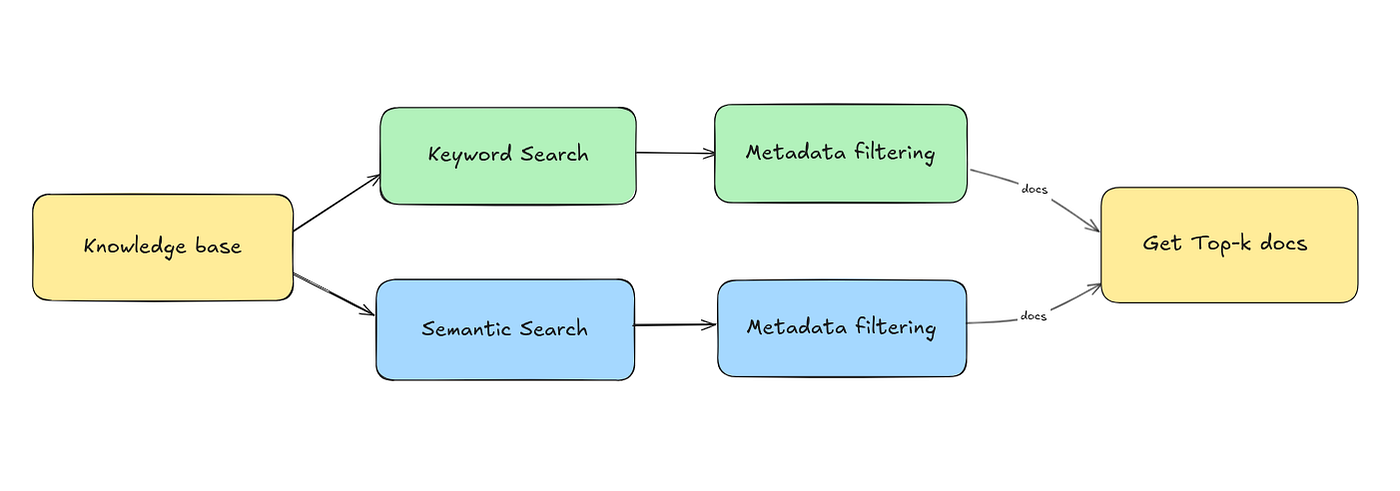
Modern Production Retrieval System (image by author)

After either search path, you typically apply a metadata filter, a post-retrieval step that prunes results based on attributes like date, source, category, or document type. The filter doesn’t change how search works; it just narrows which results survive.

When both paths are combined and the results are merged, this architecture is called Hybrid Search, the most common pattern in production RAG systems.

Metadata Filtering

Before diving into the scoring algorithms, it’s worth understanding what metadata filtering is and isn’t.

Metadata filtering is rule-based. It uses rigid criteria based on document attributes, things like author, publication date, document type, topic tags — not the content of the query.

• It doesn’t perform retrieval on its own — it narrows down results from other techniques
• It operates on user attributes, not query content
• It’s rigid, strict, fast, and easy to implement
• Conceptually simple and completely content-agnostic

Think of it like a database WHERE clause sitting on top of your vector search. You might semantic-search for “machine learning ops best practices” but then filter to only documents from the last 6 months, or only from internal engineering wikis. The semantic search finds what’s relevant; the filter enforces your constraints.

Keyword Search

When your query hits a keyword search system, it doesn’t “understand” your question — it looks for documents that share the same words. Both the query and every document in your index are represented as sparse vectors: massive arrays where the vast majority of values are zero, and only positions corresponding to terms that actually exist in the document are non-zero.

This is fundamentally different from semantic search. There’s no meaning, no context, no inference, but just term overlap. And yet, for the right use cases (exact product names, error codes, function signatures, technical jargon), it’s hard to beat.

The family of scoring algorithms that power keyword search sits under the umbrella of TF-IDF — Term Frequency, Inverse Document Frequency. Let’s build intuition from first-principle thinking.

1. Term Matching

The most naive version of keyword search builds a term-document matrix. Rows are terms, columns are documents. Each cell is 1 if the term appears in that document, 0 if it doesn’t.

Say your query is: “deploy model to production server”

Image by author

Doc A wins. But there’s an immediate problem: a document that mentions “deploy” once scores identically to one that walks through an entire deployment workflow. The frequency of occurrence is completely ignored. Let’s move a step further.

2. Term Frequency (TF)

To fix this, we move from binary presence/absence to counting how often a term appears — normalized by document length so longer documents don’t get an unfair advantage.

A 500-word document mentioning “deploy” 5 times gets a TF of 0.01(5/500). A 10,000-word document mentioning it twice gets 0.0002. Length normalization kicks in, and the shorter, focused document wins on this term.

3. Inverse Document Frequency (IDF)

TF alone still has a flaw. Words like “the”, “is”, “for”, “a” appear in almost every document. If your query contains these, every document gets a boost, which is meaningless noise.

IDF penalizes terms that are common across the corpus, and rewards rare, informative ones.

Walk through a concrete example. Say you’re indexing 200 engineering runbooks, and the word “container” appears in 8 of them:

1. Document Frequency: DF = 8/200 = 0.04
2. Flip(as it is the inverse of DF) to reward rarity: 1/0.04 = 25
3. Compress with log: log(25) ≈ 1.4

Now take the word “the” — appears in all 200 docs: IDF = log(200/200) = log(1) = 0 It contributes absolutely nothing. This is the intended behaviour.

4. TF-IDF: Putting it Together

The final score for a term in a document is simply:

image by the author

You compute this for every query term across every document, and the document with the highest sum wins. Let’s take the same example again, but for TF-IDF calculation:

image by the author

Where TF-IDF falls short:

• Zero semantic understanding — “restart service” and “reboot process” are treated as completely different queries
• Sparse representation, conceptual similarity doesn’t exist in this space

5. BM25: The Production Upgrade

Raw TF-IDF has two systematic failure modes that make it rough to run in production. BM25 (Best Matching 25) fixes both, which is why virtually every mature retrieval system uses it under the hood — Elasticsearch, OpenSearch, Solr all default to BM25.

Problem 1: Term Frequency Saturation In TF-IDF, a document mentioning “Kubernetes” 20 times scores exactly 2× a document mentioning it 10 times. At some point, extra occurrences shouldn’t keep adding proportional relevance; the document is clearly about the topic, no need to keep rewarding repetition.

BM25 applies a saturation curve. After a certain frequency, the score flattens. The document gets credit for being term-dense, but diminishing returns kick in.

Problem 2: Document Length Normalization TF-IDF penalises long documents heavily. A comprehensive 15-page architecture doc that covers your topic in depth can lose to a 1-page doc that barely mentions it, just because the TF ratio is lower in the longer doc. BM25 normalises more gently.

The formula for BM25 is:

This score is computed per keyword. You sum across all query terms to get the total relevance score for a document. Let’s take the same example and do some comparison for TF-IDF and BM25.

BM25 is the default. When engineers say “keyword search” in the context of a production system, they almost always mean BM25.

But here’s where keyword search hits a hard ceiling. Like TF-IDF, BM25 doesn’t know that “restart the service” and “reboot the process” mean the same thing. It doesn’t know that “out of memory” and “OOM error” are the same problem. It operates purely on character-level term overlap — if the exact string isn’t there, the document doesn’t score for it. You can tune k₁ and b all day, and it still won’t help you when your users query in natural language and your documents were written in technical jargon, or vice versa.

This is the fundamental gap that keyword search cannot close: it matches on form, not meaning.

To close that gap, you need a completely different representation of text — one where “restart the service” and “reboot the process” land close together in space, not because they share words, but because they share intent. That’s exactly what semantic search does. Instead of sparse term vectors, it works with dense vectors — compact numerical representations that encode meaning. And the way similarity is computed changes entirely.

Semantic Search

The core idea: represent both documents and queries as dense vectors in a shared embedding space, then measure similarity scores between those vectors. A dense vector is the opposite of a sparse TF-IDF vector — instead of a massive array that’s mostly zeros, it’s a compact array (typically 384 to 1536 dimensions depending on the model) where every single value carries information.

When you pass a sentence through an embedding model, you get back something like:

These two sentences share zero keywords. But their vectors are nearly identical, because the embedding model has learned they describe the same situation. That’s the entire value proposition of semantic search.

The Vector Space: What it actually means

Think of the vector space as a giant coordinate system with hundreds of dimensions. Every piece of text gets a unique address in that space. The key property: texts with similar meaning cluster together.

So in a well-trained embedding space:

• “deploy to Kubernetes” and “push to k8s cluster” sit close together
• “database migration script” and “schema update query” sit close together
• “quarterly budget review” sits far away from both of the above

Documents are embedded once, upfront, and stored. When a query comes in at runtime, it gets embedded on the fly, and the system finds the stored document vectors that are closest to the query vector.

How Similarity is Measured

Once you have two vectors, you need a way to measure how close they are. There are two main approaches:

Euclidean Distance Straight-line distance between two points in vector space — the same distance formula you used in high school geometry, extended to hundreds of dimensions:

Lower distance = more similar. Ranges from 0 (identical) to infinity.

The problem with Euclidean distance in high-dimensional spaces: it’s sensitive to the magnitude of vectors. Two documents about the same topic, one short, one long, might produce vectors of different magnitudes even if they point in the same general direction. That magnitude difference inflates their distance score unfairly.

Cosine Similarity Instead of measuring the distance between two points, cosine similarity measures the angle between two vectors. A small angle means they’re pointing in the same direction, so the same meaning. A large angle means they’re pointing away from each other, so a different meaning.

The denominator normalizes by the magnitude of both vectors, which is exactly what fixes the length problem. Two vectors pointing in the same direction score 1.0 regardless of whether one vector is twice as long as the other.

Range: -1 to +1

• +1 → identical direction, same meaning
• 0 → perpendicular, unrelated
• -1 → opposite directions, opposite meaning

In practice, most embedding models are trained with cosine similarity as the target metric, and most vector databases (Pinecone, Weaviate, Qdrant, Chroma) default to it. Unless you have a specific reason to use Euclidean distance, cosine similarity is the standard choice

How Embedding Models are Trained

Embedding models are trained on positive pairs (semantically similar text) and negative pairs (semantically dissimilar text).

The training loop:

1. Embed both items in a pair
2. Compute a score based on their similarity
3. Update parameters to pull positive pairs closer, push negative pairs farther apart

This is called Contrastive Learning. The model learns that “restart the service” and “reboot the process” should be close in vector space, while “restart the service” and “quarterly revenue report” should be far apart.

Important operational notes:

Semantic vectors are abstract before training, locations in vector space have no inherent meaning

You can only compare vectors from the same embedding model, mixing models produces nonsense similarity scores

Hybrid Search

Neither keyword nor semantic search is universally better. Keyword search wins for exact terminology (product names, error codes, specific function names). Semantic search wins for conceptual queries and paraphrased questions.

Hybrid search combines ranked results from both. The challenge: the scores from keyword search (BM25 values) and semantic search (cosine similarities) live on completely different scales. You can’t just add them.

Reciprocal Rank Fusion (RRF) RRF is the standard solution. Instead of trying to combine raw scores, it throws them away and only works with ranks — the position of each document in each list.

The intuition: if a document is ranked highly in both keyword and semantic search, it’s very likely relevant. RRF rewards documents for consistently appearing near the top across multiple lists.

Where k is a smoothing constant, typically set between 30 and 100. Its job is to reduce the dominance of the very top positions — without it, rank 1 would contribute an outsized score compared to rank 2.

Key properties of RRF:

• Rank-only — it doesn’t care about the actual similarity scores, just positions
• Lower k → top-ranked documents dominate more aggressively
• Scale-invariant — works regardless of how scores were originally computed

Beta: Weighting Semantic vs Keyword Beyond RRF, many systems add a beta parameter to weight the two search modes:

• β = 0.8 → Semantic search contributes 80%, keyword 20%
• β = 0.2 → Heavier keyword weighting

When to tune beta:

• If exact keyword matching is critical (product codes, technical identifiers, version numbers) → lower beta
• If conceptual understanding matters more (general knowledge questions, paraphrased queries) → higher beta

Evaluating Retrieval

You’ve built your retrieval pipeline. How do you know it works? You need retrieval quality metrics. Every evaluation setup has three components:

1. Test prompts: the queries you’re evaluating against
2. Ranked results: the documents your retriever returns, in order
3. Ground truth: a labelled dataset where each document is marked as relevant or not relevant for each query

Precision and Recall

Precision asks: “Of everything I returned, how much was actually useful?” Recall asks: “Of everything that was useful, how much did I actually find?”

There’s always a tradeoff. Retrieving more documents improves recall but hurts precision. In practice, you evaluate at a cutoff top-k, typically k = 5 to 15, because you’re only feeding a limited context window to your LLM.

MAP@k: Mean Average Precision MAP@k is more nuanced than raw precision. Instead of measuring precision once at the cutoff, it:

1. Adds precision only at positions where relevant documents appear
2. Then divides by the number of relevant documents

This rewards retrievers that surface relevant docs early in the ranking, not just somewhere in the top-k.

MRR: Mean Reciprocal Rank MRR measures how quickly your retriever finds the first relevant document.

MRR is particularly useful when you only need one good document — for example, question-answering tasks where one authoritative answer exists.

Summary

The deeper insight is that information retrieval is fundamentally a problem of representation. How you represent a document as a sparse term vector, as a dense embedding, as a set of metadata attributes — determines what kinds of similarity your system can even detect. No single representation captures everything, which is exactly why hybrid systems exist. When your retrieval is failing, the question to ask is not “should I switch to a better LLM?” but “is my representation of this content rich enough to surface it for this query?” That reframe — from generation problem to representation problem — is what separates engineers who debug RAG systematically from those who are just guessing.