Probability

Revision Notes on Probability

Photo by Edge2Edge Media on Unsplash

The following are quick notes that can be revised and revisited to check your knowledge.

If you are a non-member, please click *here*

Types of Experiments

A deterministic experiment is one where the outcome is completely predictable before it happens. Given the same conditions, you always get the same result. Example: dropping a ball from a height — it always falls down. Boiling water at 100°C at sea level — it always boils.

A random experiment is one where the outcome cannot be predicted with certainty, even if you know all the conditions. Example: tossing a coin, rolling a die, measuring the exact height of a randomly chosen person. The key feature is that there is more than one possible outcome, and which one occurs is uncertain.

The study of probability is entirely concerned with random experiments.

Types of Statistical Studies

Descriptive statistics summarise and describe the data you already have. It doesn’t try to go beyond the data. Tools include the mean (average), median (middle value), mode (most frequent), standard deviation (spread), and graphs like histograms. Example: “The average marks of our class is 74 out of 100.”

Inferential statistics uses a sample to make predictions or draw conclusions about a larger population. It involves uncertainty, so probability is central to it. Example: A poll surveys 1,000 people to predict who will win an election across millions of voters. A doctor uses a sample of patients to test whether a new drug works for all patients.

The key distinction: descriptive = describe what you have; inferential = conclude something beyond what you have.

Population and Sample

The population is the complete set of all observations or individuals you are interested in. It could be finite (all students in a school) or infinite (all possible coin tosses).

A sample is a subset drawn from the population, used because examining the entire population is often impractical, too costly, or impossible.

For a sample to be useful, it must be representative — it should reflect the diversity of the population. A biased sample leads to wrong conclusions. Example: to estimate average income in a city, surveying only people at a luxury mall gives a biased sample.

The goal of inferential statistics is to use the sample to say something reliable about the population.

Counting Principles

These are the foundational tools for calculating the number of ways things can happen — which is essential for computing probabilities.

Multiplication principle: If a task has k independent steps, with n₁ ways to do step 1, n₂ ways to do step 2, and so on, the total number of ways to complete the whole task is n₁ × n₂ × … × nₖ. Example: A menu has 3 starters, 4 mains, and 2 desserts. Total meal combinations = 3 × 4 × 2 = 24.

Without replacement: If you select k objects from n distinct objects in order and don’t put them back, the number of ways is n × (n−1) × (n−2) × … × (n−k+1). Example: Assigning 1st, 2nd, 3rd prizes from 10 contestants = 10 × 9 × 8 = 720.

Addition principle: If you can do task A in n₁ ways or task B in n₂ ways, and these are mutually exclusive (can’t do both), total ways = n₁ + n₂. Example: Travel from Delhi to Mumbai by train (5 options) or by flight (3 options) = 8 total ways.

Subtraction principle: Instead of counting what you want directly, count everything and subtract what you don’t want. This is especially useful when the phrase “at least one” appears. Example: passwords of at least one digit = (all passwords) − (passwords with no digits).

Division principle: When every valid arrangement is counted exactly k times in your total count, divide by k to get the actual count. Example: The word KARNATAKA has 9 letters with A repeated 4 times and K repeated 2 times, so arrangements = 9! / (4! × 2!) = 7560.

Permutations and Combinations

Permutation counts the number of ways to arrange objects where order matters.

The number of ways to arrange all n distinct objects is n! (n factorial) = n × (n−1) × … × 2 × 1. Example: Arrange A, B, C = 3! = 6: ABC, ACB, BAC, BCA, CAB, CBA.

The number of ordered selections of r objects from n distinct objects is:

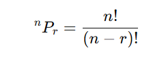
Permutation formula

Example: 3-letter words from {A, B, C, D} = 4P3 = 4!/1! = 24.

Combination counts selections where order does not matter. Choosing {A, B} is the same as {B, A}.

Combination formula

Example: Choosing 2 students from {A, B, C} = 3C2 = 3: {A,B}, {A,C}, {B,C}.

Key properties:

Key properties of combinations

Combination with repetition: Choosing r items from n types where repetition is allowed and order doesn’t matter =

Example: Choose 3 fruits from apple, banana, orange with repetition = C(5,3) = 10 ways.

Balls and boxes: Distributing n identical balls into k distinct boxes (any box can have any number) =

This is the “stars and bars” formula. Example: 4 identical balls into 3 boxes = C(6,2) = 15 ways.

Functions

A function f: X → Y assigns exactly one element of Y (the output) to each element of X (the input). X is the domain, Y is the co-domain, and the set of actual outputs is the range (which may be smaller than Y).

Injective (one-to-one): Different inputs always give different outputs. No two elements of X map to the same element of Y. Formally: if f(a) = f(b), then a = b. Example: f(x) = 2x is injective. f(x) = x² is not injective because f(2) = f(−2) = 4.

The number of injective functions from a set of m elements to a set of n elements (where n ≥ m) is n × (n−1) × … × (n−m+1) = nPm.

Surjective (onto): Every element of Y is the image of at least one element of X. The range equals the co-domain. Example: f(x) = x³ from R to R is surjective because every real number has a cube root. f(x) = x² from R to R is not surjective because negative numbers are never outputs.

Bijective: Both injective and surjective. This means there is a perfect pairing between X and Y. Only bijective functions have an inverse function f⁻¹: Y → X. Example: f(x) = x + 3 is bijective on R, with inverse f⁻¹(y) = y − 3.

Set Theory

A set is an unordered collection of distinct elements, written in curly braces: A = {1, 2, 3}.

Two sets are equal (A = B) if and only if they contain exactly the same elements — equivalently, A ⊆ B and B ⊆ A simultaneously.

The universal set Ω contains all possible elements under consideration. Every set in the discussion is a subset of Ω.

Set operations:

• Union A ∪ B: everything in A or B (or both)
• Intersection A ∩ B: everything in both A and B
• Complement Aᶜ: everything in Ω not in A
• Difference A \ B: in A but not in B

De Morgan’s Laws are essential for simplifying complements of unions and intersections:

Example: A = {1,2,3}, B = {3,4,5}, Ω = {1,2,3,4,5,6}. (A∪B)ᶜ = {6} = {4,5,6} ∩ {1,2,6} .

The power set P(A) is the set of all subsets of A, including ∅ and A itself. If |A| = n, then |P(A)| = 2ⁿ. Example: A = {a, b} → P(A) = {∅, {a}, {b}, {a,b}}, which has 4 elements.

Sample Space and Events

The sample space S (or Ω) is the set of all possible outcomes of a random experiment. Example: tossing two coins → S = {HH, HT, TH, TT}.

An event is any subset of the sample space. It can be a single outcome (simple event) or a collection of outcomes (compound event). Example: event “at least one head” = {HH, HT, TH}.

Disjoint (mutually exclusive) events: A ∩ B = ∅. They cannot both occur in the same trial. Example: rolling a 3 and rolling a 5 on one die toss are mutually exclusive.

Collectively exhaustive events: E₁ ∪ E₂ ∪ … ∪ Eₙ = Ω. At least one of them must occur. Example: {even, odd} is collectively exhaustive for a die roll.

A partition of Ω is a collection of events that are both mutually exclusive and collectively exhaustive — they cover everything with no overlap.

Continuous sample spaces arise when outcomes are measurements rather than discrete values. Example: the exact time a bus arrives could be any value in [0, 60] minutes — uncountably many outcomes. Events become intervals, and we cannot assign probability to individual points.

Probability Basics

For a random experiment with equally likely outcomes:

P(A) = (number of favourable outcomes) / (total number of outcomes)

Example: rolling a fair die, P(even) = 3/6 = 0.5.

Axioms of probability (Kolmogorov):

• P(A) ≥ 0 for any event A
• P(Ω) = 1
• For disjoint events A and B: P(A ∪ B) = P(A) + P(B)

From these axioms, everything else follows:

Complement rule: P(Aᶜ) = 1 − P(A). Example: P(not rolling a 6) = 1 − 1/6 = 5/6.

Inclusion-exclusion:

The intersection is subtracted because it gets counted twice. Example: P(A) = 0.4, P(B) = 0.5, P(A ∩ B) = 0.2 → P(A ∪ B) = 0.7.

For disjoint events P(A ∩ B) = 0, so P(A ∪ B) = P(A) + P(B) simply.

Conditional Probability

The conditional probability P(A|B) is the probability of event A occurring given that event B has already occurred. Knowing B has happened restricts the sample space to B.

provided P(B) > 0.

Example: A card is drawn from a standard deck. A = “it’s a king”, B = “it’s a face card”. P(A ∩ B) = P(king) = 4/52. P(B) = 12/52. So P(king | face card) = (4/52)/(12/52) = 4/12 = 1/3. There are 4 kings among 12 face cards.

Conditional addition rule: If A and C are mutually exclusive given B, then P(A ∪ C | B) = P(A|B) + P(C|B).

Conditional probability satisfies all the same axioms as regular probability — it’s just probability within a restricted universe.

Chain Rule (Multiplication Rule)

The chain rule lets you compute joint probabilities by chaining conditional probabilities.

Also,

Both forms are equivalent — use whichever is easier to compute.

Example: A bag has 5 red and 3 blue balls. You draw two without replacement. P(both red) = P(1st red) × P(2nd red | 1st red) = (5/8) × (4/7) = 20/56 ≈ 0.357.

The chain rule extends to more events:

P(A ∩ B ∩ C) = P(A) · P(B|A) · P(C|A∩B)

Example: Drawing 3 red balls from the same bag = (5/8) × (4/7) × (3/6) = 60/336 ≈ 0.179.

Law of Total Probability

If events B₁, B₂, …, Bₖ form a partition of Ω (mutually exclusive and exhaustive), then for any event A:

This lets you compute the overall probability of A by breaking the sample space into cases.

Example: A factory has three machines. Machine 1 produces 50% of items with a 1% defect rate. Machine 2 produces 30% with a 3% defect rate. Machine 3 produces 20% with a 5% defect rate.

P(defective) = 0.50 × 0.01 + 0.30 × 0.03 + 0.20 × 0.05 = 0.005 + 0.009 + 0.010 = 0.024

So 2.4% of all items are defective.

Think of it as a weighted average of conditional probabilities, weighted by how likely each scenario is.

Bayes’ Theorem

Bayes’ theorem lets you reverse a conditional probability — going from P(E|H) to P(H|E). It’s the formal way to update your beliefs when new evidence arrives.

Bayes Theorem

where P(E) is computed using the law of total probability.

Terminology:

• Prior P(H): your belief in hypothesis H before seeing evidence
• Likelihood P(E|H): how probable the evidence is if H is true
• Posterior P(H|E): updated belief in H after seeing evidence E

Example (classic medical test): A disease affects 1% of the population. A test is 95% sensitive (P(+|disease) = 0.95) and 95% specific (P(−|no disease) = 0.95, so P(+|no disease) = 0.05).

You test positive. What’s the probability you actually have the disease?

P(+) = P(+|disease)·P(disease) + P(+|no disease)·P(no disease) = 0.95 × 0.01 + 0.05 × 0.99 = 0.0095 + 0.0495 = 0.059

P(disease|+) = (0.95 × 0.01) / 0.059 ≈ 0.161

Only about 16%! This counterintuitive result comes from the disease being rare. Most positive tests come from the large healthy population, not the small sick population. This is why mass screening programs require highly specific tests.

Independence

Two events A and B are independent if knowing one occurred gives no information about the other.

Formally:

Equivalently: P(A|B) = P(A) and P(B|A) = P(B).

Example: Flip two coins. P(H on 1st) = 0.5, P(H on 2nd) = 0.5, P(both H) = 0.25 = 0.5 × 0.5 . The coins don’t affect each other.

Important: Mutually exclusive events (P(A ∩ B) = 0) are almost never independent (unless one has probability 0). If A and B are disjoint and both have positive probability, then P(A ∩ B) = 0 ≠ P(A)·P(B) > 0. In fact, knowing A occurred tells you B definitely didn’t — they are as dependent as possible.

Three-way independence requires all four conditions simultaneously:

• P(A ∩ B) = P(A)P(B)
• P(A ∩ C) = P(A)P(C)
• P(B ∩ C) = P(B)P(C)
• P(A ∩ B ∩ C) = P(A)P(B)P(C)

Pairwise independence does not imply mutual independence. You need the four-way condition explicitly.

Conditional independence: A and B are conditionally independent given C if P(A ∩ B | C) = P(A|C) · P(B|C). Two events can be independent unconditionally but dependent given C, or vice versa (Simpson’s paradox territory).

Random Variables

A random variable X is a function that maps each outcome in the sample space to a real number. It converts a qualitative outcome into a numerical quantity we can do arithmetic with.

Example: Toss two coins. Outcomes: {HH, HT, TH, TT}. Define X = number of heads. Then X(HH) = 2, X(HT) = 1, X(TH) = 1, X(TT) = 0. X is a random variable.

Discrete random variables take values from a countable set. Their distribution is described by the probability mass function (PMF):

Properties: Pₓ(x) ≥ 0 for all x, and Σ Pₓ(x) = 1 (probabilities sum to 1).

For the coin example: P(X=0) = 1/4, P(X=1) = 2/4 = 1/2, P(X=2) = 1/4. Sum = 1.

Continuous random variables take values from an interval or the whole real line.

Bernoulli Distribution

The simplest distribution: only two outcomes, called success (1) and failure (0).

where p ∈ [0,1] is the success probability.

Mean: E[X] = p.

Variance: Var(X) = p(1−p).

The variance is maximised at p = 0.5 (most uncertainty) and is zero at p = 0 or p = 1 (no uncertainty).

Example: A quality check on a product: defective with probability 0.04, non-defective with probability 0.96. X = 1 (defective), X = 0 (non-defective). E[X] = 0.04 (4% defect rate). Var = 0.04 × 0.96 = 0.0384.

The Bernoulli distribution is the building block for the Binomial.

Binomial Distribution

X ~ Binomial(n, p) counts the number of successes in n independent Bernoulli trials, each with success probability p.

The term C(n,k) counts the number of ways to place k successes in n trials. pᵏ is the probability of k successes, (1−p)^(n−k) is the probability of the remaining n−k failures.

Mean: np.

Variance: np(1−p).

Example: A call center agent successfully resolves 70% of calls. In 10 calls:

P(exactly 7 resolved) = C(10,7) · 0.⁷⁷ · 0.³³ = 120 × 0.0824 × 0.027 ≈ 0.267

Mean = 10 × 0.7 = 7 calls resolved. Variance = 10 × 0.7 × 0.3 = 2.1, so σ ≈ 1.45.

P(at least 8) = P(X=8) + P(X=9) + P(X=10) — here the subtraction principle helps: 1 − P(X ≤ 7).

Poisson Distribution

X ~ Poisson(λ) models the count of rare, independent events occurring in a fixed interval of time or space, where λ is the average rate.

for k = 0, 1, 2, …

Mean: λ.

Variance: λ. (Mean equals variance — a distinctive property.)

Example: A website gets an average of λ = 3 visitors per minute. The number of visitors in any given minute follows Poisson(3).

P(0 visitors) = e⁻³ ≈ 0.050 P(exactly 3) = e⁻³ · ³³ / 3! = 0.050 × 27 / 6 ≈ 0.224 P(more than 5) = 1 − P(X ≤ 5) ≈ 1 − 0.916 = 0.084

The Poisson distribution is a limiting case of the Binomial when n is large, p is small, and λ = np. So it’s useful when you have many trials (millions of people) with a low probability of each (probability of a particular disease).

Geometric Distribution

X ~ Geometric(p) models the number of trials needed until the first success, where each trial has success probability p independently.

for x = 1, 2, 3, …

This says: x−1 failures followed by 1 success.

Mean: 1/p.

Variance: (1−p)/p².

The memoryless property: P(X > m + n | X > m) = P(X > n). If you’ve already failed m times, the distribution of remaining trials is the same as if you were starting fresh. The geometric distribution is the only discrete distribution with this property.

Example: You roll a die until you get a 6 (p = 1/6). Mean rolls = 1/(1/6) = 6. P(first 6 on 4th roll) = (5/6)³ × (1/6) ≈ 0.096. P(need more than 6 rolls) = P(X > 6) = (5/6)⁶ ≈ 0.335.

Multinomial Distribution

The multinomial generalises the Binomial to more than two outcomes. In n trials, each trial results in one of k outcomes with probabilities p₁, p₂, …, pₖ (summing to 1).

where x₁ + x₂ + … + xₖ = n.

Example: A die has faces 1–6, each with probability 1/6. Roll 12 times. What’s the probability each face appears exactly twice?

P = 12! / (2!⁶) × (1/6)¹² = 479001600 / 64 × (1/6)¹² ≈ 0.0034

Only about a 0.34% chance — fair dice rarely produce perfectly even distributions in small samples.

The multinomial coefficient n!/(x₁!…xₖ!) counts the number of ways to arrange n objects where type i appears xᵢ times — it’s a generalisation of the division principle from topic 4.

Discrete Uniform Distribution

Every outcome in {a, a+1, …, b} is equally likely.

for each x in that range.

Mean: (a+b)/2.

Variance: ((b−a+1)² − 1)/12.

Example: A fair die gives a=1, b=6. P(any face) = 1/6. Mean = 3.5. Variance = (36−1)/12 = 35/12 ≈ 2.92.

This is the discrete version of “no information” — you have no reason to favour any outcome over another. Many games, lotteries, and randomisation procedures assume a uniform distribution.

Expectation

The expected value E[X] is the long-run average value of X over many independent repetitions of the experiment. It is a weighted average of all possible values, weighted by their probabilities.

Example: A game pays ₹10 if you roll a 6 and ₹0 otherwise. E[winnings] = 10 × (1/6) + 0 × (5/6) = ₹1.67 per game. If you pay ₹2 to play, you lose money on average.

Linearity of expectation is extremely powerful:

The second property holds even when the random variables are dependent. This is what makes it easy to derive the mean of the Binomial: X = X₁ + … + Xₙ where each Xᵢ ~ Bernoulli(p), so E[X] = nE[X₁] = np.

Variance

Variance measures the spread of a distribution around its mean — how much values typically deviate from E[X].

The shortcut formula is often easier to compute:

Example: Fair die. E[X] = 3.5. E[X²] = (1 + 4 + 9 + 16 + 25 + 36)/6 = 91/6 ≈ 15.17. Var = 15.17 − 3.⁵² = 15.17 − 12.25 = 2.92.

Properties of variance:

• Var(aX + b) = a²·Var(X) (shifting by b doesn’t change spread; scaling by a scales variance by a²)
• Var(X + Y) = Var(X) + Var(Y) + 2·Cov(X,Y)
• If X and Y are independent: Var(X + Y) = Var(X) + Var(Y)

Variance is always non-negative. A variance of zero means X is a constant (no randomness at all).

Standard Deviation

Standard deviation is in the same units as X, which makes it more interpretable than variance. If X is measured in kilograms, Var(X) is in kg² (awkward), but σ is in kg (natural).

Example: Exam scores with mean 70 and σ = 10. A score of 85 is 1.5 standard deviations above the mean. For many distributions, roughly 68% of values fall within 1σ of the mean, and 95% within 2σ (the empirical rule, exact for normal distributions).

Standard deviation answers the question: “How far from the mean should I typically expect a random observation to be?”

Covariance

Covariance measures how two random variables vary together.

Positive covariance: X and Y tend to be above their means together and below together. Example: height and weight.

Negative covariance: When X is above its mean, Y tends to be below its mean. Example: temperature and hot chocolate sales.

Zero covariance: No linear relationship. Independence implies zero covariance, but zero covariance does not imply independence (there could be a non-linear relationship).

Properties:

• Cov(X,X) = Var(X)
• Cov(aX, bY) = ab·Cov(X,Y)
• Cov(X+Y, Z) = Cov(X,Z) + Cov(Y,Z)

Covariance depends on the scale of X and Y, making it hard to compare across different pairs of variables. That’s what correlation fixes.

Correlation

Correlation is a normalised version of covariance:

It always lies between −1 and 1.

• ρ = 1: perfect positive linear relationship (X and Y move together exactly)
• ρ = −1: perfect negative linear relationship
• ρ = 0: no linear relationship

Example: ρ between outdoor temperature and ice cream sales might be 0.85 (strong positive). ρ between study hours and number of errors might be −0.70 (strong negative). ρ between shoe size and exam score might be near 0.

Crucial warning: Correlation measures only linear relationships. Two variables can have ρ = 0 and still be strongly related in a non-linear way. Also, correlation does not imply causation — ice cream sales and drowning rates are positively correlated (both driven by hot weather), but ice cream doesn’t cause drowning.

PDF — Probability Density Function

For continuous random variables, individual outcomes have probability zero (P(X = 3.7) = 0). Instead, probability is spread over intervals, described by the PDF f(x).

Properties: f(x) ≥ 0 for all x,

The probability that X falls in the interval [a, b]:

This is the area under the density curve between a and b.

Example: Uniform distribution on [0, 1]: f(x) = 1 for 0 ≤ x ≤ 1, and 0 elsewhere. P(0.2 ≤ X ≤ 0.7) = 0.7 − 0.2 = 0.5.

Exponential distribution with rate λ: f(x) = λe^(−λx) for x ≥ 0. This models waiting times — the time until the next bus, the lifetime of a light bulb. Mean = 1/λ.

The PDF itself is not a probability (it can exceed 1). Only integrals of f give probabilities.

CDF — Cumulative Distribution Function

The CDF gives the probability that X takes a value ≤ x:

Fₓ(x) = P(X ≤ x)

For discrete variables:

For continuous variables:

The CDF is always non-decreasing, starts at 0 as x → −∞, and reaches 1 as x → +∞.

Finding probability between two points:

Example: Standard normal distribution (mean 0, σ = 1). F(1.96) ≈ 0.975. F(−1.96) ≈ 0.025. So P(−1.96 ≤ Z ≤ 1.96) = 0.975 − 0.025 = 0.95. This is the origin of the “95% confidence interval” concept.

For discrete variables, the CDF is a step function — it jumps at each possible value of X by the probability of that value. The derivative of a continuous CDF is the PDF: f(x) = F’(x).

Conclusion

In this article, some basic concepts of probability are discussed.

Thank you to all the readers for your valuable time! If you like the content, please clap and subscribe, as I will try to post other content related to data science soon.