How To Use Custom Or Official YOLOv8 Object Detection Model In ONNX Format

In this article, we’ll see how to use any pretrained or custom YOLOv8 object detection model in a well known open format known as ONNX (Open Neural Network Exchange). Utilizing this format offers an advantage that it can be used in deployment in multiple programming languages without depending on official Ultralytics module.

In this write up, I’ll use official YOLOv8n model available here but the method will also be applicable to any custom YOLOv8 model converted to ONNX format.

First of all we need to convert our trained model with .pt extension to onnx format using the following code.

from ultralytics import YOLO

model_path = 'path/to/yolov8n.pt'

model = YOLO(model_path)

model.export(format='onnx', opset = 12, imgsz =[640,640])

Ensure you have already installed the ultralytics module before running the above code. Once the onnx file is generated, we can define all the classes that our model can detect. In my case, it is the pre-trained model trained over coco dataset and can identify 80 classes.

with open('coco-classes.txt') as file:
    content = file.read()
    classes = content.split('\n')

del classes[-1]

print(classes) # Let's print classes list

The above code snippet on execution gives the following output,

['person', 'bicycle', 'car', 'motorbike', 'aeroplane', 'bus', 'train', 'truck', 'boat', 'traffic light', 'fire hydrant', 'stop sign', 'parking meter', 'bench', 'bird', 'cat', 'dog', 'horse', 'sheep', 'cow', 'elephant', 'bear', 'zebra', 'giraffe', 'backpack', 'umbrella', 'handbag', 'tie', 'suitcase', 'frisbee', 'skis', 'snowboard', 'sports ball', 'kite', 'baseball bat', 'baseball glove', 'skateboard', 'surfboard', 'tennis racket', 'bottle', 'wine glass', 'cup', 'fork', 'knife', 'spoon', 'bowl', 'banana', 'apple', 'sandwich', 'orange', 'broccoli', 'carrot', 'hot dog', 'pizza', 'donut', 'cake', 'chair', 'sofa', 'pottedplant', 'bed', 'diningtable', 'toilet', 'tvmonitor', 'laptop', 'mouse', 'remote', 'keyboard', 'cell phone', 'microwave', 'oven', 'toaster', 'sink', 'refrigerator', 'book', 'clock', 'vase', 'scissors', 'teddy bear', 'hair drier', 'toothbrush']

For inference, we can read the image using OpenCV.

# read the image
image = cv2.imread('bicycle.jpg')

# YOLOv8 need RGB image
img = cv2.cvtColor(image,cv2.COLOR_BGR2RGB)
img_height,img_width = img.shape[:2]

Since OpenCV read image in BGR format whereas YOLO expects an RGB format, so we converted our image into RGB and also store image dimensions for later use. But that’s not all! Before YOLO can work its magic, there are some additional image processing required. Let’s take a look at the image’s shape.

print(img.shape)

(420, 620, 3)

Our image is a 3 channel RGB image with width and height of 620 and 420 respectively. In Contrast, our YOLOv8 model expect an image of size (640, 640) and the channel information before the image size.

# resize image to get the desired size (640,640) for inference
img = cv2.resize(img,(640,640))

# change the order of image dimension from (640,640,3) to (3,640,640)
img = img.transpose(2,0,1)

Finally, to feed the dnn module with our image we need an extra dimension at the 0th index that tells the module how many images we are providing at a time. Additionally, our image pixels range from 0 to 255. They must be scaled to change this range to 0–1 before inference.

# add an extra dimension at index 0
img = img.reshape(1,3,640,640)

# scale to 0-1
img = img/255.0

Finally, our image is ready for inference. To run the inference with our onnx model we can use readNetFromONNX() or readNet() method from DNN module.

# read the trained onnx model
net = cv2.dnn.readNetFromONNX('yolov8n.onnx')  # readNet() also works

# feed the model with processed image
net.setInput(img)

# run the inference
out = net.forward()

After running the inference we obtain an output matrix containing the model’s predictions as shown in above code. To understand how to extract the valuable information it holds, let’s first print the shape of this output matrix.

print(out.shape)

(1, 84, 8400)

The matrix shape of (1, 84, 8400) indicates 8400 detections each with 84 parameters. This is because our YOLOv8 model is designed to always predict up to 8400 objects in an image. It’s important to note that not all detections will be accurate, we’ll need to filter based on confidence scores later. Here 84 at the first index corresponds to the number of parameters for each detection. This includes the bounding box coordinates (x1, y1, x2, y2) and confidence scores for 80 different classes. This structure might differ for custom models. The number of confidence scores depends on the number of classes your model is trained on. For example, if YOLOv8 is trained to detect 1 class, there would be 5 parameters instead of 84. For 2 classes there will be 6 on the first index and so on. We can simply remove the 1 at 0th index as it just tells that a single image being processed by model.

results = out[0]

Now transposing the matrix to get the shape (8400, 84) for our ease.

results = results.transpose()

As mentioned above, each detection includes a confidence score for each class. To identify the class an object or detection most likely belongs to, we simply find the class with the highest confidence score. Additionally, to remove the detections with all the confidences lower than given threshold we can use the following function.

def filter_Detections(results, thresh = 0.5):
    # if model is trained on 1 class only
    if len(results[0]) == 5:
        # filter out the detections with confidence > thresh
        considerable_detections = [detection for detection in results if detection[4] > thresh]
        considerable_detections = np.array(considerable_detections)
        return considerable_detections

    # if model is trained on multiple classes
    else:
        A = []
        for detection in results:

            class_id = detection[4:].argmax()
            confidence_score = detection[4:].max()

            new_detection = np.append(detection[:4],[class_id,confidence_score])

            A.append(new_detection)

        A = np.array(A)

        # filter out the detections with confidence > thresh
        considerable_detections = [detection for detection in A if detection[-1] > thresh]
        considerable_detections = np.array(considerable_detections)

        return considerable_detections

results = filter_Detections(results)

Once we get the useful result by excluding useless parameters, we can print the shape to better understand our results.

print(results.shape)

(45, 6)

Looks like now we have 45 detections each having 6 parameters. They are bounding box top left (x1, y1) and bottom right (x2, y2) coordinates, class id and confidence value. Before we go ahead, let’s have a look on the picture i run the inference on.

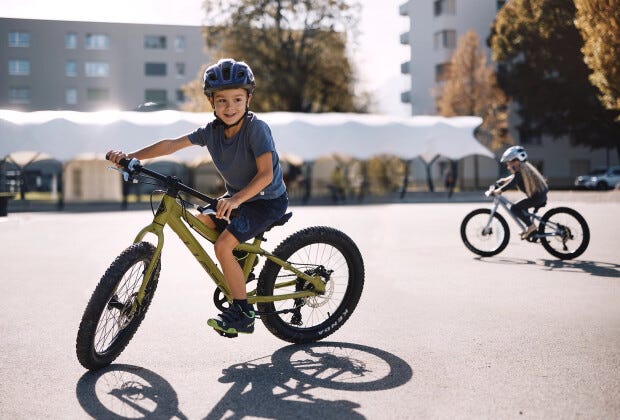
Looking at this picture one can easily tells that this picture does not contains 45 objects at all. The reason our resultant matrix still containing so many detections because multiple detections pointing to same object. To address this, we can apply a well known technique called Non-Maximum Suppression (NMS). NMS acts as a filter, selecting the best detections among those potentially referring to the same object. It achieves this by considering two key metrics which are confidence value (how certain the model is about the detection) and Intersection over Union (IOU). Additionally, we’ll need to rescale the remaining detections back to their original scale. This is because our model has output the detection for an image of size 640x640 which is not the size of our original image.

def NMS(boxes, conf_scores, iou_thresh = 0.55):

    #  boxes [[x1,y1, x2,y2], [x1,y1, x2,y2], ...]

    x1 = boxes[:,0]
    y1 = boxes[:,1]
    x2 = boxes[:,2]
    y2 = boxes[:,3]

    areas = (x2-x1)*(y2-y1)

    order = conf_scores.argsort()

    keep = []
    keep_confidences = []

    while len(order) > 0:
        idx = order[-1]
        A = boxes[idx]
        conf = conf_scores[idx]

        order = order[:-1]

        xx1 = np.take(x1, indices= order)
        yy1 = np.take(y1, indices= order)
        xx2 = np.take(x2, indices= order)
        yy2 = np.take(y2, indices= order)

        keep.append(A)
        keep_confidences.append(conf)

        # iou = inter/union

        xx1 = np.maximum(x1[idx], xx1)
        yy1 = np.maximum(y1[idx], yy1)
        xx2 = np.minimum(x2[idx], xx2)
        yy2 = np.minimum(y2[idx], yy2)

        w = np.maximum(xx2-xx1, 0)
        h = np.maximum(yy2-yy1, 0)

        intersection = w*h

        # union = areaA + other_areas - intesection
        other_areas = np.take(areas, indices= order)
        union = areas[idx] + other_areas - intersection

        iou = intersection/union

        boleans = iou < iou_thresh

        order = order[boleans]

        # order = [2,0,1]  boleans = [True, False, True]
        # order = [2,1]

    return keep, keep_confidences

def rescale_back(results,img_w,img_h):
    cx, cy, w, h, class_id, confidence = results[:,0], results[:,1], results[:,2], results[:,3], results[:,4], results[:,-1]
    cx = cx/640.0 * img_w
    cy = cy/640.0 * img_h
    w = w/640.0 * img_w
    h = h/640.0 * img_h
    x1 = cx - w/2
    y1 = cy - h/2
    x2 = cx + w/2
    y2 = cy + h/2

    boxes = np.column_stack((x1, y1, x2, y2, class_id))
    keep, keep_confidences = NMS(boxes,confidence)
    print(np.array(keep).shape)
    return keep, keep_confidences

Applying the above functions on our result.

rescaled_results, confidences = rescale_back(results, img_width, img_height)

Here ‘rescaled_results’ contains the bounding box (x1, y1, x2, y2) and class id while ‘confidences stores’ the corresponding confidence scores.

Finally we are ready to visualize these results on our image.

for res, conf in zip(rescaled_results, confidences):

    x1,y1,x2,y2, cls_id = res
    cls_id = int(cls_id)
    x1, y1, x2, y2 = int(x1), int(y1), int(x2), int(y2)
    conf = "{:.2f}".format(conf)
    # draw the bounding boxes
    cv2.rectangle(image,(int(x1),int(y1)),(int(x2),int(y2)),(255,0,255),1)
    cv2.putText(image,classes[cls_id]+' '+conf,(x1,y1-17),
                cv2.FONT_HERSHEY_SCRIPT_COMPLEX,1,(255,0,255),1)