Brain Age Prediction Using Graph Neural Networks on Structural Connectomes

By Cyprien Rivier and Claire Tang as part of the Stanford CS224W course project.

1. Introduction

1.1 The Concept of Brain Age

Magnetic resonance imaging (MRI) can be used to estimate how “old” a brain appears relative to a person’s chronological (or “true”) age. In brain-age prediction, a model is trained to map neuroimaging data to chronological age and the model’s output is the predicted brain age. The difference between the predicted brain age and chronological age, called the brain-age gap or brain-age delta, can contain valuable information about the health and resilience of the brain.

The idea is that, if the model is good enough at predicting chronological age, when the model predicts an older brain age than the chronological age, it’s because it picked up on features that are usually associated with older brains. And vice-versa for very healthy brains, where the predicted brain age is younger than the chronological age.

It has been shown multiple times that individuals whose brains appear “older” than expected (positive brain-age gap) have higher risk of mortality, cognitive decline, and incident neurodegenerative disease, like Alzheimer’s disease [1]. Therefore, brain-age models can serve as useful biomarkers to guide brain health interventions across the lifespan.

1.2 Why Graph Neural Networks?

Traditional approaches to brain-age prediction either extract handcrafted features from images (like regional volumes or cortical thickness) or apply convolutional neural networks directly to the 3D brain scans [2]. While these methods work reasonably well, they don’t naturally capture the relational structure of brain networks. A voxel-based CNN treats the brain as a regular 3D grid, but it cannot capture the organization of the brain as a network, since it is not aware of its underlying anatomical connections.

GNNs have been applied to brain connectivity data only relatively recently, with initial work focusing on functional connectivity for disease classification tasks [3, 4]. For brain-age prediction specifically, a few studies have explored GNN-based approaches using functional connectivity or structural connectomes [5]. However, most of these studies use relatively small datasets (hundreds of subjects) and don’t systematically compare different GNN architectures or graph construction choices.

We propose here to explore graph neural networks to predict brain age from structural brain graphs derived from diffusion MRI tractography, and determine what are the important elements for successful predictions.

1.3 Structural Brain Graphs

The brain can be naturally represented as a network: gray-matter regions form the nodes, and the white-matter fiber bundles connecting them form the edges. This representation, called the structural connectome, captures how different brain areas are wired together [6].

Importantly, this network organization is not random: the brain exhibits characteristic properties like small-world topology (high local clustering with efficient global communication), hub regions that act as communication centers (similar to big airports acting as hubs for international flights), and modular structure where densely connected groups of regions support specific functions [7, 8].

These network properties change with age. Older brains tend to show decreased communication efficiency, weakening of hub connectivity, and reduced integration between distant regions. Therefore, the structural connectome is a promising target for brain-age prediction. Let’s see if we can use graph neural networks to capture these changes and predict brain age!

2. Methods

2.1 Data

Our sample includes 10,000 subjects from the UK Biobank [9], ranging from 45 to 82 years old. We do not impose any restriction on the age distribution of the sample or inclusion criteria for the participants.

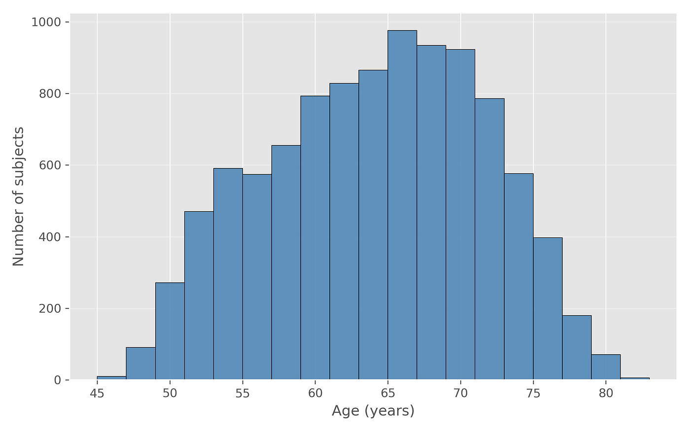
Age distribution of our 10,000 subjects

2.2 Diffusion MRI and Tractography

Diffusion MRI data captures how water molecules diffuse in brain tissue [10]. In white matter, water diffuses preferentially along axon bundles because cell membranes and myelin sheaths constrain movement in the other directions. This directional preference (anisotropy) can be exploited to reconstruct white-matter pathways through a process called tractography [11]. For each subject, tractography produces a dense collection of white matter fibers, each represented as a polyline in 3D running between two gray-matter voxels. These fibers will be used to construct the edges of our brain graphs.

2.3 Brain Parcellation

To define the nodes of our brain graphs, we have to divide the cortex into regions based on a predefined atlas. We considered several atlases: Glasser (360 regions) [12] and the Schaefer atlases (100, 300, 500, 800regions) [13]. We also added subcortical regions from the Melbourne Subcortex Atlas (Tian) at two scales: S1 with 16 regions and S4 with 54 regions [14]. Combining cortical and subcortical parcellations gives us brain graphs ranging from 116 nodes to 854 nodes.

2.4 Brain Graph Construction

We built undirected brain graphs where nodes are grey matter brain regions and edges are white-matter connections. We defined an edge between two regions if at least one streamline connects them.

Brain graph construction. Created with Biorender.com

2.4.1 Node Features: We considered degree (number of connections), strength (sum of edge weights), clustering coefficient (how connected a node’s neighbors are to each other), eigenvector centrality (importance based on connections to other important nodes), and participation coefficient (diversity of connections across network modules) [15]. These features capture both local connectivity patterns and each node’s role in the global network. Below is our Python implementation of the participation coefficient (which first requires to partition the nodes into distinct modules).

def modularity(A, gamma=1):
    """
    Produces a subdivision of the network into
    nonoverlapping groups of nodes in a way that maximizes the number of
    within-group edges, and minimizes the number of between-group edges.
    The modularity quantifies the degree to which the 
    network can be subdivided into such groups.

    Inputs:
        W,
            undirected weighted or binary connection matrix
        gamma,
            resolution parameter
                gamma>1,        detects smaller modules
                0<=gamma<1,     detects larger modules
                gamma=1,        classic modularity

    Outputs:    
        Ci     optimal community structure
        Q      maximized modularity
    """
    N = len(A)  # number of nodes
    K = np.sum(A, axis=0)  # degree
    m = np.sum(K)  # number of edges
    B = A - gamma * np.outer(K, K) / m  # modularity matrix
    Ci = np.ones(N, dtype=int)  # module indices
    cn = 1  # number of modules
    U = [1, 0]  # array of unexamined modules

    ind = np.arange(N)
    Bg = B.copy()
    Ng = N

    while U[0]:  
        e_vals, e_vecs = np.linalg.eig(Bg)
        i1 = np.argmax(np.real(e_vals))  # maximal positive eigenvalue of Bg
        v1 = e_vecs[:, i1]  # corresponding eigenvector

        S = np.ones(Ng, dtype=int)
        S[v1 < 0] = -1
        q = S.T @ Bg @ S  # contribution to modularity

        if q > 1e-10:  # contribution positive: U(1) is divisible
            qmax = q  # maximal contribution to modularity
            Bg[np.eye(Ng, dtype=bool)] = 0 
            indg = np.ones(Ng, dtype=bool)  # array of unmoved indices
            Sit = S.copy()
            while np.any(indg):  # iterative fine-tuning
                Qit = qmax - 4 * Sit * (Bg @ Sit)  # recompute Qit
                if np.all(np.isnan(Qit[indg])) or not np.any(indg):  # break loop if all values are NaN or indg is all False
                    break

                imax = np.argmax(Qit[indg])
                imax = np.arange(Ng)[indg][imax]  # find original index
                Sit[imax] *= -1
                indg[imax] = False
                if not np.any(indg):
                    break
                if np.nanmax(Qit[indg]) > q:
                    q = np.nanmax(Qit[indg])
                    S = Sit.copy()

            if abs(np.sum(S)) == Ng:  # unsuccessful splitting of U(1)
                U.pop(0)
            else:
                cn += 1
                Ci[ind[S == 1]] = U[0]  # split old U(1) into new U(1) and into cn
                Ci[ind[S == -1]] = cn
                U = [cn] + U
        else:  # contribution nonpositive
            U.pop(0)

        if len(U) == 1 and U[0] == 0:  # termination condition
            break

        ind = np.where(Ci == U[0])[0] 
        bg = B[ind, :][:, ind]
        Bg = bg - np.diag(np.sum(bg, axis=0))  # modularity matrix
        Ng = len(ind)  # number of vertices in U(1)

    s = Ci[:, np.newaxis] 
    Q = np.sum(~(s - s.T) * B / m)
    return Ci, Q

def participation_coef(W, Ci, flag=0):
    """
    Parameters:
    W, binary or weighted, directed or undirected connection matrix
    Ci, community affiliation vector (from modularity)
    flag, 0, undirected graph (default)
    1, directed graph: out-degree
    2, directed graph: in-degree

    Returns:
    P, participation coefficient
    """

    if flag == 2:
        W = W.T

    n = len(W)  # number of vertices
    Ko = np.sum(W, axis=1)  # degree
    Gc = (W != 0) @ np.diag(Ci)  # neighbor community affiliation
    Kc2 = np.zeros(n)  # community-specific neighbors

    for i in range(1, np.max(Ci) + 1):
        Kc2 += np.square(np.sum(W * (Gc == i), axis=1))

    epsilon=1e-10 # Avoid division by zero
    P = np.ones(n) - Kc2 / np.square(Ko + epsilon)
    P[Ko == 0] = 0  # P=0 for nodes with no (out)neighbors

    return P

2.4.2 Edge Features: We computed multiple edge weight metrics. In addition to the number of white matter tracts connecting two regions, we also computed several microstructural metrics averaged along the streamlines connecting each region pair:

• Fractional Anisotropy (FA): Measures how directionally constrained diffusion is; sensitive to myelination and axonal density
• Mean/Axial/Radial Diffusivity (MD, AD, RD): Measure overall and directional diffusion rates; sensitive to tissue integrity
• Free Water (FW): Estimates extracellular water fraction; increases with atrophy
• NODDI metrics (ICVF, ISOVF, OD): Model-based estimates of neurite density, free water, and fiber dispersion
• Mean Signal Kurtosis (MSK): Captures non-Gaussian diffusion; reflects tissue complexity

The purpose of these metrics is to capture the health or quality of the white matter fibers, in addition to their raw number.

2.5 Graph Sparsification

Raw connectome matrices are quite dense since most region pairs have at least some connecting streamlines, including artifacts from the tractography process. It is therefore necessary to sparsify the graph to focus on the most meaningful connections and make GNNs learn better. We considered two sparsification methods: top-k sparsification and density-based sparsification.

For top-k sparsification, we keep only the k strongest connections for each node. If an edge is in the top-k for either node, it is kept. We used k = 40 as the default, which keeps the primary projection targets for each region while substantially reducing the number of edges.

For density-based sparsification, we keep the strongest edges until we reach a certain fraction of the total number of edges. We used a density of 0.1 as the default, which retains 10% of total possible edges and yields a similar density as top-k sparsification with k = 40.

3. Experiments

3.0 General Strategy

Already at the graph construction stage, there are many knobs that can be tuned (graph size, sparsification method, sparsification threshold). To avoid exploding the search space, we start by fixing one balanced graph construction strategy: the Glasser + Tian S4 parcellation (414 nodes) with density-based sparsification at density 0.1. At the end of the experiments, we will come back to this choice and explore the impact of different graph construction strategies on the performance of the model.

We held out 1,000 subjects (10%) as a fixed test set that was never used during model development. The remaining 9,000 subjects were split into training (~8,100) and validation (~900) sets.

We report Mean Absolute Error (MAE) as the primary metric, along with R² and Pearson correlation between predicted and true age. We use MAE as our loss metric, but the Pearson correlation is necessary to assess the quality of the model, since it is robust to scale and directly measures how well the model captures age-related variation (whereas MAE depends on the initial age distribution).

3.1 Phase 1: Baseline GCN

We began with a standard Graph Convolutional Network (GCN) [16] as our baseline. The initial model used 3 layers with 128 hidden dimensions, mean pooling for graph-level readout, dropout (p=0.2), graph normalization, and no node features beyond the graph structure itself.

With this baseline, we got a Pearson correlation of just 0.05 and MAE of 6.24 years. The model had essentially no predictive power, suggesting that the graph topology alone was not containing any useful information.

By adding node features derived from the graph structure (degree, strength, clustering coefficient, eigenvector centrality, and participation coefficient), we achieved a correlation of 0.47 and MAE of 5.46 years, which is encouraging and showed that the data actually contained usable signal.

GCN (3 layers, 128 hidden dim) using all node features

3.2 Phase 2: GraphSAGE

To improve the performance of the baseline GCN, we then tested increasing the GCN hidden dimensions up to 256, achieving a correlation of 0.51 and MAE of 5.30, only a marginal improvement. This showed that model capacity was not the bottleneck and that the model was not underfitting, leading us to explore different GNN architectures.

By switching to GraphSAGE [17] (which separately processes a node’s own embedding and its neighbors’ embeddings before combining them), we achieved a correlation of 0.64 and MAE of 4.57 years, a significant jump forward.

GraphSAGE (3 layers, 256 hidden_dim)

Let’s look at the formulas to understand this improvement. GCN computes node updates using a normalized adjacency matrix:

GCN update formula

Where Ã= A + I, D is its degree matrix, H are node features, and W is a learnable weight matrix. GCN mixes neighbor and self embeddings with the same transformation, which can blur node identity and lead to oversmoothing. On the other hand, GraphSAGE (mean) separates the two types of embeddings, with distinct learnable weight matrices for self and neighbors:

GraphSAGE update formula

Therefore, by treating differently the self and neighbor embeddings in its update, GraphSAGE is able to preserve a region’s “identity”, and it is likely that certain aging-related features are region-specific.

3.3 Phase 3: Edge Attributes as first-class citizens

Up to this point, our models were not properly using edge attributes. The edge weight is used to some degree in GCN to scale messages, but our best model so far, GraphSAGE, is not using them at all. However, a lot of relevant information is present in the edge attributes we have constructed, which contain microstructural metrics (FA, MD, NODDI, etc) that describe the quality of each white matter connection.

To better leverage the information in the edges, we moved to GINE (Graph Isomorphism Network with Edge features) [18, 19], an architecture that explicitly incorporates edge attributes into the message passing process. Instead of simply aggregating neighbor features, GINE modulates messages based on edge attributes:

GINE update formula

where e represents the edge features and W is a linear map projecting the edge features onto the dimension of the node embeddings.

The code for GINE is:

import torch
import torch.nn as nn
import torch.nn.functional as F
from torch_geometric.nn import GINEConv, GraphNorm, global_add_pool

class GINERegressor(nn.Module):
    """
    Graph Isomorphism Network with Edge features for regression.

    Parameters:
    in_channels : int
        Number of input node features.
    edge_dim : int
        Number of edge features.
    hidden_channels : int
        Hidden dimension for all layers.
    num_layers : int
        Number of GINE layers.
    dropout : float
        Dropout probability.
    out_channels : int
        Output dimension (1 for regression).
    """

    def __init__(
        self,
        in_channels: int,
        edge_dim: int = 0,
        hidden_channels: int = 256,
        num_layers: int = 3,
        dropout: float = 0.2,
        out_channels: int = 1,
    ):
        super().__init__()
        if num_layers < 1:
            raise ValueError("num_layers must be >= 1")

        self.edge_dim = edge_dim
        self.dropout = dropout

        # Projection of input to hidden dimension
        self.input_proj = nn.Linear(in_channels, hidden_channels)

        # GINE layers
        self.convs = nn.ModuleList()
        self.norms = nn.ModuleList()

        for _ in range(num_layers):
            # MLP for GINEConv aggregation
            mlp = nn.Sequential(
                nn.Linear(hidden_channels, hidden_channels),
                nn.ReLU(),
                nn.Linear(hidden_channels, hidden_channels),
            )
            conv = GINEConv(mlp, edge_dim=edge_dim if edge_dim > 0 else None)
            self.convs.append(conv)
            self.norms.append(GraphNorm(hidden_channels))

        # Prediction head
        self.readout = nn.Linear(hidden_channels, out_channels)

    def forward(self, data):
        """
        Forward pass.

        Parameters:
        data : torch_geometric.data.Data
            Graph data with attributes:
            - x: Node features [num_nodes, in_channels]
            - edge_index: Edge connectivity [2, num_edges]
            - edge_attr: Edge features [num_edges, edge_dim]
            - batch: Batch assignment [num_nodes]

        Returns:
        torch.Tensor
            Predicted values [batch_size].
        """
        x, edge_index = data.x, data.edge_index
        edge_attr = getattr(data, "edge_attr", None)
        batch = getattr(data, "batch", None)

        # Handle edge_attr based on edge_dim
        if self.edge_dim == 0:
            edge_attr = None

        # Handle single graph case (no batch tensor)
        if batch is None:
            batch = torch.zeros(x.size(0), dtype=torch.long, device=x.device)

        # Input projection
        x = self.input_proj(x)

        # GINE layers
        for conv, norm in zip(self.convs, self.norms):
            x = conv(x, edge_index, edge_attr=edge_attr)
            x = norm(x, batch)
            x = F.relu(x)
            x = F.dropout(x, p=self.dropout, training=self.training)

        # Global pooling (sum)
        hg = global_add_pool(x, batch)

        # Prediction
        out = self.readout(hg).squeeze(-1)
        return out

This architecture change led to a very significant improvement in performance. With GINE using all 13 edge attributes (FA, MD, AD, RD, FW, NODDI metrics, MSK, and streamline counts), correlation jumped to 0.76 and MAE dropped to 3.80 years. The R² reached 0.57, meaning the model now explained more than half the variance in age.

GINE (3 layers, 256 hidden_dim)

This is the confirmation that the “quality” of white matter connections, and not just their presence, is very relevant for predicting brain age, and taking it into account reduced error by nearly a full year compared to our best topology-only models.

3.3.1 Note on GINE vs GAT

We tried GAT (Graph Attention Network), which can also use the information contained in the edge attributes. The result was better than GraphSAGE, but worse than GINE, with a correlation of 0.69 and a MAE of 4.34 years.

GAT (3 layers, 256 hidden_dim)

To understand, let’s recall the GAT update:

GAT update

where the α (attention coefficients) are defined as:

GAT attention coefficients

The main difference between GINE and GAT regarding edge features handling is that GAT uses the edge features to inform the attention scores, but the aggregation itself is only based on node features. As we saw above, GINE is able to directly incorporate the edge features in its messages to shape how information flows between nodes, allowing to better use the microstructure information contained in the edge attributes.

3.3.2 Note on GINE vs GIN

To make sure that the performance gain came from the edge attributes and not from the MLP of GINE’s update, we tested standard GIN (Graph Isomorphism Network) [18], the same architecture as GINE but without edge attributes.

GIN update

GINE update

We found that GIN performed significantly worse than GINE, with a correlation of 0.61 and a MAE of 4.73 years, confirming that GINE is strictly superior for our connectome data where the edge attributes are biologically meaningful.

GIN (3 layers, 256 hidden_dim)

3.4 Phase 4: Sparsity Sweep

With GINE established as our best architecture, we were then interested in exploring different levels of sparsity in the graph, first based on the density-based sparsification method:

Graph density vs performance

We notice improvements as we make the graph denser, up to a certain point. There seems to be an optimal density around 0.14, with higher densities leading to worsening performance. It’s likely that weaker connections are artifactual and adding them is providing more noise than signal.

However, the results also show that sparse graphs worked remarkably well. With density set to 0.08 (keeping only the top 8% of the total number of possible edges), we still achieved correlation of 0.75 and MAE of 3.9 years, quite close to much denser graphs. This suggests that the strongest connections carry the primary age-related predictive signal, and weaker connections are only adding finer details to further refine the predictions.

We also tested the other sparsity method: top-k sparsification, which retains the k strongest connections for each node.

Top-k parameter vs performance

It’s worth noting that this sweep was much narrower since top_k = 30 ~ density = 0.07 and top_k = 70 ~ density = 0.17 We thus observe a similar trend as in the density sweep, where adding more edges lead to better performance for relatively sparse graphs.

3.5 Phase 5: Graph Resolution Sweep

Then, we explored various graph resolutions by using different parcellations. As a reminder, we have considered several atlases to parcellate the cortex, which yielded graphs of different sizes: ranging from 116 nodes (Schaefer 100 + Tian S1) to 854 nodes (Schaefer 800 + Tian S4). All our experiments so far were done with the Glasser + Tian S4 parcellation (414 nodes).

Graph size vs performance

We found that there is a significant gain in performance when moving from low resolution (100 parcels) to medium-high resolution (500 parcels). This suggests that coarse parcellations average out meaningful local microstructural variation that is crucial for age prediction.

We also notice diminishing returns, and increasing resolution further does not provide additional benefit. It is possible that the graph becomes too noisy and that the added spatial granularity does not provide signal relevant to brain aging.

3.6 Phase 6: Edge Features Ablation

Since most of our gains came from the edge attributes, a natural question is to determine the importance of each type of edge attribute on the performance of the model. This is also relevant to understanding which biomarker of white matter health is most important for predicting brain age.

Ablation of Edge Features

The results confirm that microstructural features are the primary driver of performance, outperforming standard connectome weights (streamline counts and SIFT2-derived counts). Specifically, NODDI metrics (ICVF, ISOVF, OD) seem to contain the most dense predictive signal, as models using only NODDI features achieved almost the same performance as the model using all features.

This suggests that for brain age prediction, the tissue microstructure integrity (captured by NODDI) is more informative than the macro-scale fiber density (captured by streamline and SIFT2 counts) or simple DTI metrics. Adding other microstructural measures (like DTI or Free Water) to NODDI did not really improve performance, suggesting they are providing redundant information.

4. Conclusion

In summary, our results show that using GNNs on structural connectomes can capture meaningful patterns of brain aging, especially when using microstructural edge attributes, sufficiently fine parcellations, and the right graph density. The GINE architecture achieved the best performance, highlighting the value of the edge features in brain graphs derived from tractography.

Even if our initial experiments do not yet outperform previous models on brain age prediction, it is a promising direction since it is based on a different type of information than existing methods (pattern of structural connections between brain regions vs images or functional connectivity). We can imagine future approaches that fuse information from different modalities (T1, structural connectivity, functional connectivity) to improve prediction accuracy, where a GNN based on structural brain connectivity would be one module integrated in a multimodal pipeline.

5. References

Github repository.

[1] Gaser C, et al. BrainAGE in mild cognitive impaired patients: predicting the conversion to Alzheimer’s disease. PLoS ONE. 2013.

[2] Cole JH, Franke K. Predicting age using neuroimaging: innovative brain ageing biomarkers. Trends in Neurosciences. 2017.

[3] Ktena SI, et al. Metric learning with spectral graph convolutions on brain connectomes. NeuroImage. 2018.

[4] Parisot S, et al. Disease prediction using graph convolutional networks: application to autism spectrum disorder and Alzheimer’s disease. Medical Image Analysis. 2018.

[5] Stankevičiūtė K, et al. Population graph GNNs for brain age prediction. MLCN Workshop, MICCAI. 2020.

[6] Sporns O, Tononi G, Kötter R. The human connectome: a structural description of the human brain. PLoS Computational Biology. 2005.

[7] Bassett DS, Bullmore ET. Small-world brain networks. The Neuroscientist. 2006.

[8] van den Heuvel MP, Sporns O. Network hubs in the human brain. Trends in Cognitive Sciences. 2013.

[9] Sudlow C, et al. UK Biobank: an open access resource for identifying the causes of a wide range of complex diseases of middle and old age. PLoS Medicine. 2015.

[10] Le Bihan D, et al. Diffusion tensor imaging: concepts and applications. Journal of Magnetic Resonance Imaging. 2001.

[11] Mori S, van Zijl PCM. Fiber tracking: principles and strategies — a technical review. NMR in Biomedicine. 2002.

[12] Glasser MF, et al. A multi-modal parcellation of human cerebral cortex. Nature. 2016.

[13] Schaefer A, et al. Local-global parcellation of the human cerebral cortex from intrinsic functional connectivity MRI. Cerebral Cortex. 2018.

[14] Tian Y, et al. Topographic organization of the human subcortex unveiled with functional connectivity gradients. Nature Neuroscience. 2020.

[15] Rubinov M, Sporns O. Complex network measures of brain connectivity: uses and interpretations. NeuroImage. 2010.

[16] Kipf TN, Welling M. Semi-supervised classification with graph convolutional networks. ICLR. 2017.

[17] Hamilton WL, Ying R, Leskovec J. Inductive representation learning on large graphs. NeurIPS. 2017.

[18] Xu K, et al. How powerful are graph neural networks? ICLR. 2019.

[19] Hu W, et al. Strategies for pre-training graph neural networks. ICLR. 2020.