Appendix: Mathematical Details for “Post-War Advances in Survey Sampling”

This appendix gives the mathematical details behind the estimators discussed in the main article. It collects the formulae and assumptions behind the Horvitz–Thompson estimator, PPS multi-stage sampling, sample rotation, replication-based variance estimation, and calibration weighting.

A. The Horvitz-Thompson Estimator

Figure 1: (Left) Morris H. Hansen (1910–1990) — His papers with William N. Hurwitz in the 1940s are viewed as foundational building blocks for the theory of multi-stage sampling with unequal probabilities (U.S. Census Bureau). (Right) Daniel G. Horvitz (1921–2008) — He (together with Donovan J. Thompson) co-authored in 1952 a research paper that introduced what was later called the Horvitz-Thompson estimator, which provided a general framework for unequal-probability sampling.

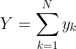
Consider a finite population U = {1, 2,…, N} with a study variable y taking values y₁, y₂,…, yN​. The parameter of interest is the population total:

Under a probability sampling design p(.), each unit k has first-order inclusion probability:

where s denotes the selected sample.

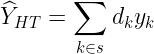
The Horvitz-Thompson (HT) estimator of Y is:

where dₖ = 1/πₖ​ is the design weight of unit k.

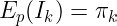
Let Iₖ​ be the sample-membership indicator for unit k. Then

Therefore,

Thus, the estimator is design-unbiased provided πₖ > 0 for all units.

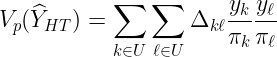
Let

be the second-order inclusion probability, and define

The design variance of the HT estimator is:

For fixed-size without-replacement designs, the Sen-Yates-Grundy variance estimator is

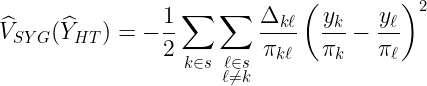
This form assumes a fixed-size without-replacement design with positive second-order inclusion probabilities for sampled pairs.

B. Multi-Stage Sampling with PPS at the First Stage

Suppose the population is partitioned into M primary sampling units, or PSUs. PSU i contains Nᵢ secondary units, and its population total is

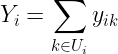
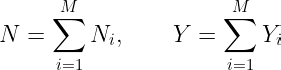
The total population size and total of y are

With-replacement PPS: Hansen-Hurwitz estimator

Suppose m PSUs are drawn independently with replacement, with selection probabilities ​p₁, …, pᴍ​, where

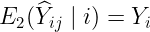
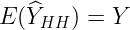
If PSU i is selected at draw j, let Ŷᵢⱼ​ be an unbiased estimator of Yᵢ from the second-stage sample, so that

The Hansen-Hurwitz estimator is

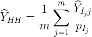
where Iⱼ is the PSU selected on draw j.

This estimator is unbiased:

Let

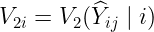
be the second-stage variance when PSU i is selected.

Then the variance is

The first term is the between-PSU component; the second is the contribution from second-stage sampling within PSUs.

Self-weighting PPS design

For a without-replacement first-stage PPS design, suppose the first-order inclusion probability of PSU i is

assuming ​πᵢ ≤ 1.

If a simple random sample of fixed size n₀​ is drawn within each selected PSU, then the conditional probability of selecting secondary unit k within PSU i is

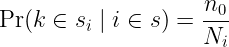
The overall inclusion probability of a secondary unit in PSU i is therefore

Thus, all secondary units have the same inclusion probability before later adjustments (see caveat), giving an idealised self-weighting design.

Caveat: This derivation abstracts from certainty PSUs, stratification, frame imperfections, nonresponse, and later calibration adjustments.

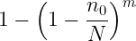
For with-replacement PPS, the same expression is best interpreted as the expected number of selections across draws. The probability of being selected at least once is not exactly mn₀​​/N, but rather

C. Rotation and Replication

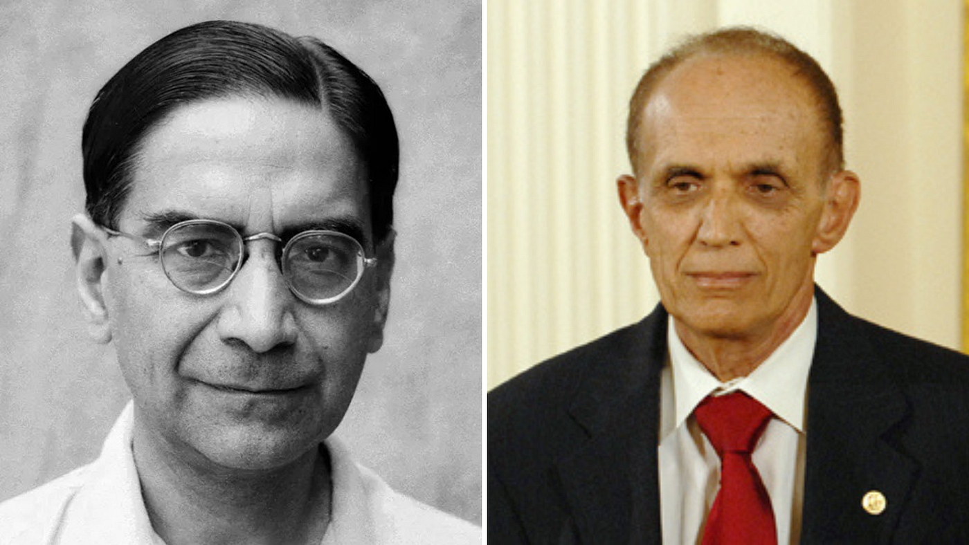
Figure 2: (Left) Prasanta C. Mahalanobis (1893–1972) — He developed the technique of interpenetrating subsampling (also known as replicated sampling) in his crop surveys of the 1930s, setting it out fully in 1946 (Wikimedia Commons). (Right) Bradley Efron (1938– ) — The bootstrap resampling technique proposed by him in 1979 was one of the first computer-intensive statistical techniques and has had a major impact on the field (Wikimedia Commons).

Rotation groups and direct estimation

At time t, let

be the finite population.

Let yᵢₜ​ be the value of the study variable for unit i at time t. The population total and mean are

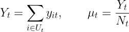
Let sₜ be the sample at time t, formed from active rotation groups, and let wᵢₜ​ be the final survey weight for sampled unit i.

The generic direct estimator of the total is

If the weights are pure Horvitz-Thompson weights, then

where πᵢₜ​ is the inclusion probability of unit i at time t.

The direct HT estimator is

Under the sampling design p(.), the estimator is unbiased

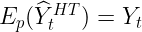
Let Aₜ​​ be the set of active rotation groups at time t. Suppose each active group r ∈ Aₜ produces an unbiased estimator Ŷᵣₜ of the same total:

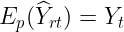
A combined estimator is

If the groups have approximately equal precision, equal weights are natural:

Then the combined estimator becomes:

Direct estimation of the mean

If Nₜ​ is known from benchmark totals, estimate the mean by

Equivalently,

If Nₜ​ is not treated as known, a common alternative is the Hájek estimator:

If group-level mean estimators μ_hatᵣₜ​ are available, then

With equal group weights,

Variance under the design

For a direct Horvitz-Thompson estimator at time t,

For the mean,

when Nₜ is known.

For a combined rotation-group estimator,

If active groups are independent and have common variance V, equal weights give

Note: In real rotating surveys, rotation groups may not be perfectly independent because of shared design features, stratification, and operational procedures.

Why rotation helps for change estimation

Let the true change be

The simplest direct estimator is

Its variance is

Rotation helps because overlapping samples usually make the covariance term positive, reducing the variance of the estimated change relative to independent cross-sections.

Matched-sample and composite estimation

In a rotating-panel design, the sample at time t can be partitioned into a matched component and an unmatched component. The matched component consists of units also present in the sample at time t − 1.

Let:

• Ŷₜꟲ be the current composite estimate,
• Ŷₜᴰ be the direct estimate from the full sample at time t,
• Ŷₜˍ₁ꟲ be the previous composite estimate,
• Ŷₜᴰ,ₘ​ be the matched-sample estimate for time t,
• Ŷₜˍ₁ᴰ,ₘ​ be the corresponding matched-sample estimate for time t − 1.

A generic composite estimator is

The bracketed term updates the previous composite estimate by adding the estimated matched-sample change. The parameter α controls the balance between the current direct estimate and the updated previous estimate. Its optimal value depends on the autocorrelation of the survey variable, the overlap fraction, and the variances of the direct and matched-sample estimators.

In operational labour-force surveys, the actual composite estimator may include additional adjustments and smoothing parameters; the expression here is a simplified generic form.

D. Variance Estimation for Complex Survey Designs

Jackknife variance estimation for stratified multi-stage designs

Consider a stratified multi-stage design with H strata, and n​ₕ PSUs selected in stratum h. Let θ_hat denote the full-sample estimate of a parameter θ.

For the delete-one-PSU jackknife:

For each stratum h = 1, …, H and each PSU j = 1, …, n​ₕ​, form the jackknife replicate by deleting PSU j from stratum h and multiplying the weights of the remaining PSUs in that stratum by

Compute the replicate estimate θ_hat(ₕⱼ)​.

A common stratified delete-one-PSU jackknife variance estimator is:

The factor (nₕ -1)/n​ₕ ensures that the estimator is approximately unbiased for the true variance for smooth (differentiable) statistics.

Equivalent replicate-scale conventions are used in different software packages.

The Rao-Wu rescaling bootstrap

Figure 3: (Left) J.N.K. Rao (1937– ) (Society of Statistics, Computer and Applications); (Right) Chien-Fu Jeff Wu (1949– ) (Wikimedia Commons): The Rao-Wu bootstrap is a specialised resampling technique used in survey statistics to estimate sampling variances for complex, multi-stage, and stratified sample designs.

For a stratified design with H strata and n​ₕ PSUs selected in stratum h, the rescaling bootstrap proceeds as follows:

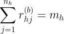
For bootstrap replicate b = 1, …, B, within each stratum h, draw a simple random sample with replacement of size mₕ from the nₕ​ PSUs. In many applications,

Let rₕⱼ(ᵇ)​ denote the number of times PSU j in stratum h is selected in bootstrap replicate b. Thus,

A general rescaled replicate weight for each unit k belonging to PSU j in stratum h can be written as:

where dₕⱼₖ​ is the original design weight. This general scaled form, with the tuning constant λₕ, is due to Rao, Wu, and Yue (1992); it extends the original Rao-Wu (1988) bootstrap.

When first-stage sampling fractions are negligible,

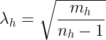
With mₕ = nₕ — 1, the replicate weight simplifies to:

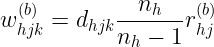
This is the common simplified Rao-Wu bootstrap weight form used in several Statistics Canada applications. If PSU j is not selected in replicate b, then rₕⱼ(ᵇ) ​= 0, and the simplified replicate weight for units in that PSU is zero before later calibration or other adjustments.

With mₕ = nₕ — 1, the rescaling ensures that E∗[wₕⱼₖ​(ᵇ)] = dₕⱼₖ (where E∗ denotes expectation under the bootstrap distribution) and that the bootstrap variance is consistent for the true design-based variance under the regularity conditions of the Rao-Wu/Rao-Wu-Yue rescaling bootstrap.

Compute the bootstrap replicate estimates θ_hat(ᵇ) using the replicate weights wₕⱼₖ​(ᵇ).

A common bootstrap variance estimator is:

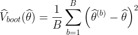
Some implementations instead centre around the mean of the bootstrap replicate estimates and use a slightly different scale factor. The correct convention depends on how the replicate weights were constructed.

E. Calibration Estimation

Figure 4: (Left) Jean-Claude Deville (1944–2021) (International Statistical Institute); (Right) Carl-Erik Särndal (1937– ) (Statistical Society of Canada): Pioneers who established the unified theoretical framework for calibration weighting and GREG estimation in survey sampling. Their work provided statisticians with flexible tools for integrating auxiliary population data to improve survey estimates.

Let xₖ = (xₖ₁, …, xₖⱼ)ᵀ be a vector of J auxiliary variables for unit k, with known population total

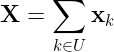
The design-weighted estimator of the auxiliary total is

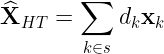
Calibration seeks new weights wₖ​ (for k ∈ s) that are close to the design weights dₖ​, while satisfying the calibration equation

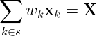
Formally, the calibration problem is

where G(w, d) is a distance function satisfying G(d, d) = 0, G(w, d) ≥ 0, and appropriate smoothness conditions.

Chi-square distance and the GREG estimator

For chi-square distance, the distance function G(w, d) is defined as:

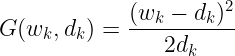
The solution yields the GREG weights:

and the resulting calibration estimator of the total of y can be written as the generalised regression estimator:

where

and

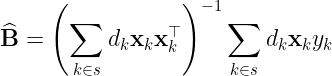
is the weighted regression coefficient. Assume that Σ d*ₖxₖxₖ*ᵀ is nonsingular; otherwise a generalised inverse or a reduced calibration model is needed.

Unlike the pure HT estimator, calibration estimators are generally not exactly design-unbiased in finite samples, but they are typically design-consistent and can be more efficient when the auxiliary variables are predictive of the study variable.

Exponential distance and raking

For the exponential distance, the distance function G(w, d) is defined as:

The resulting weights have multiplicative adjustments of the form

where λ is chosen to satisfy the calibration constraints.

When the auxiliary variables are categorical margins, this corresponds closely to classical raking or iterative proportional fitting. A key advantage is that the weights remain positive.

Asymptotic variance of the calibration estimator

Under standard regularity conditions, the calibration estimator has the same first-order asymptotic variance as the HT estimator applied to residuals.

Define the population regression residual

where B is the population regression coefficient of y on x.

A common expression for the approximate variance is

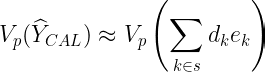
When the auxiliary variables **x**ₖ​ are strongly related to yₖ​, the residuals eₖ​ have smaller variation than the original yₖ​, and calibration can substantially improve precision relative to the unadjusted HT estimator.