The Phase Manifold Model — Spinor Extensions

Boundary Orientation, Transition Structure, and the Origin of Spin

This article extends the original Phase Manifold Model (PMM) by introducing a boundary orientation sector that accommodates spinor structure within the existing phase framework.

Core Idea

Reality evolves through a gated three-phase structure — Before (B), During (D), and After (A) — in which time is ordered by phase progression, space exists only during an active window, gravity arises from the accumulated memory of completed interactions (Φ), and spin emerges from unresolved boundary orientation encoded at phase transitions (Σ).

Phase Structure (B → D → A)

• Before (B) → probabilistic (quantum state, reversible)
• During (D) → geometric (emergent spacetime, GR)
• After (A) → informational (record, accumulation)

Key Principles

• Time is phase-ordered, not a single continuous parameter
• Space is emergent, active only within Θ_win
• Gravity arises from accumulated transition memory (Φ)
• Structural depth (δ) modifies geometry but does not source it
• Phase transitions (@) are finite-width physical regions
• Boundary twist (Ξ) encodes transition asymmetry
• Spin (Σ) is a boundary orientation effect, not intrinsic rotation

Event Flow

Ψ_B → @ → D → A → Φ → (feeds forward)

• Ψ_B → @ → D → A → Φ → (feeds forward)
• Ψ_B → @ Quantum potential in the Before phase reaches the transition region.
• P = |ψ|² defines the collapse distribution at @.
• @ → D Collapse initiates D-phase realization. Geodesics evolve in τ_D. Spacetime geometry g^(D) is active only where Θ_win ≠ 0.
• D → A Dynamics unfold within D. A is the non-spatial boundary where closure completes (Θ_out).
• A → Φ The completed B–D–A traversal is recorded in the phase-memory field Φ.
• Φ → (feeds forward) The accumulated record influences subsequent geometry and future closures.

Transition Region (@)

Transition Region (Θ_@)

The trigger/contact vertex (@) initiates realization.

This activation generates the finite-width overlap manifold Θ_@, where:

• The spacetime realization window remains active (Θ_win ≠ 0)
• Closure begins (Θ_out activates)
• Expected and realized stress-energy differ (ΔT)
• Transition write into the phase-memory field Φ occurs
• Boundary orientation (Σ) resolves

Transition write:

Γ@ · Θ@ · (ΔT)² → Φ

Derived Structures

Gate Functions

• Θ_in → opens spacetime
• Θ_out → closes spacetime

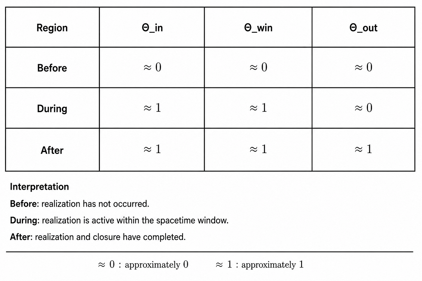
Diagram 2- Gate Logic

✔ Θ_in and Θ_out define the opening and closing of the space window, with Φ written at Θ_out and becoming active immediately in D.

Active Windows

• Θ_win = Θ_in (1 − Θ_out) → spacetime active
• Θ_@ = Θ_win Θ_out → transition region

Boundary Structures

• Twist tensor (Ξ) → antisymmetric boundary structure
• Holonomy (ℛ_@) → residual closure rotation
• Orientation field (Σ) → unresolved boundary state

Metric / Fields

Metric (Leading Order)

Spacetime exists only within Θ_win:

Where:

✔ Φ → gravitational memory ✔ δ → structural depth modifier ✔ Σ → orientation backreaction

Phase-Memory Field (Φ)

✔ Recovers GR in strong field ✔ Produces MOND-like behavior in weak field

Transition Write (Θ_@)

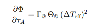
Where:

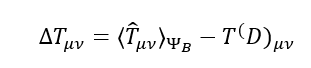
✔ Write occurs only at closure (D → A).

Boundary Twist & Holonomy

Boundary twist is generated by the relative orientation of the Θ_in and Θout gradients and is active within the Θ@ transition manifold.

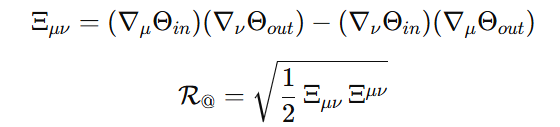
✔ Ξ encodes transition asymmetry ✔ ℛ_@ encodes closure mismatch/rotation

Spin / Orientation Sector (Σ)

This field encodes unresolved rotational structure at the transition boundary.

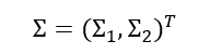
With double-cover behavior:

• Σ(2π) = −Σ
• Σ(4π) = Σ

Spin Connection (from transition structure)

Spin connection generated from the oriented misalignment between admission and closure boundaries along the local phase-flow direction.

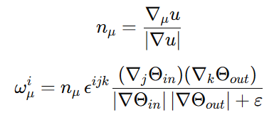
✔ This defines boundary holonomy.

Covariant Derivative

Orientation Lagrangian

Equation of Motion

Structural Depth (δ)

✔ Activates in high density + curvature ✔ Modifies geometry

Structural Depth Lagrangian (L_δ)

To promote structural depth to a dynamical quantity:

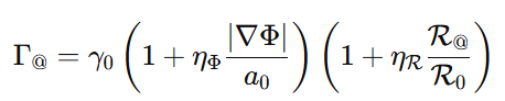
Effective Publication Rate

Geometric Overview

The following diagram integrates the phase structure, gating functions, and effective spacetime geometry into a single representation.

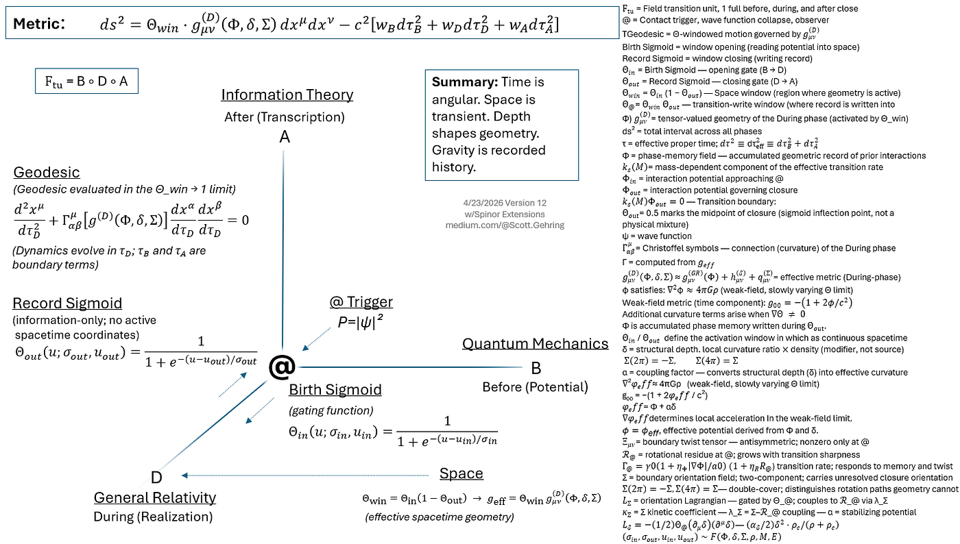
Diagram 3 — Geometric Overview

Spacetime exists only within Θwin, while gravity and orientation emerge from boundary processes localized at Θ@.

Validation

Model remains consistent with:

• Newtonian limit ✔
• GR recovery ✔
• Schwarzschild ✔
• Lensing ✔
• Galaxy rotation curves ✔
• Tully–Fisher ✔
• Solar system ✔
• Arrow of time ✔
• Measurement irreversibility ✔

Conceptual Breakthrough

Paradoxes arise from compressing B, D, and A into a single time parameter.

PMM resolves this by:

• Separating temporal roles
• Linking them through a physical transition field (FTU)
• Accumulating outcomes into Φ
• Allowing orientation (Σ) to persist beyond geometric closure

✔ Gravity = accumulated record ✔ Spin = boundary holonomy

The following diagram summarizes how transition gradients propagate through boundary twist and holonomy to produce spin behavior, providing the basis for the predictions that follow.

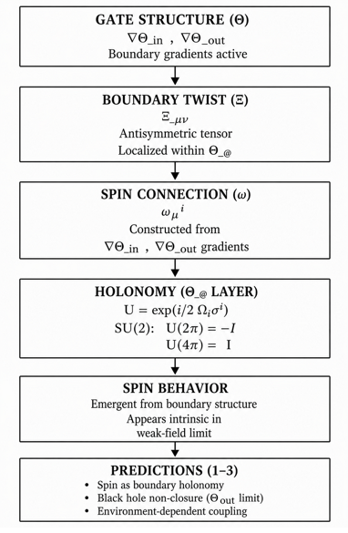
Diagram 4 — Boundary Holonomy and Spin Structure

Predictions

1. Spin Requires Transition Structure

Spin follows from the boundary holonomy structure:

• Appears intrinsic due to continuous microscopic transitions
• Dynamically tied to Θ gradients

2. Black Holes Trap Orientation

If Θ_out fails to close:

• Φ accumulates indefinitely
• Σ cannot fully resolve

✔ Black holes become spin non-closure zones

3. Spin is Environment-Dependent

Because ω depends on Θ gradients:

• stronger curvature → stronger holonomy
• predicts small corrections to:
• spin precession
• spin–orbit coupling
• spin-dependent lensing

Compact Math

═════════════════════════════════════════════════════════════
PMM COMPACT MATH
Phase Manifold Model w/Spinor Extensions — Version 9
═════════════════════════════════════════════════════════════

PHASE PROGRESS
u = local monotonic phase parameter (B → D → A)
u_in < u_out

FIELD TRANSITION UNIT (FTU)
F_tu = B ∘ D ∘ A

GAUGE LABELED COORDINATES
B = (c⁰)ₘₚ 
D = (c¹,c²)꜀ 
A = (c³)ₖᴮ

FTU COORDINATE NOTATION
Fₜᵤᶜ = (B,D,A) = ((c⁰)ₘₚ , (c¹,c²)꜀ , (c³)ₖᴮ)

FTU DYNAMICS
B[Φ] → @ → D(Θ_in → Θ_win → Θ_out) → A(Φ')

CONTACT OPERATOR
Θcon​⇒(Θin​,Θwin​,Θout​)

GATE FUNCTIONS
Θ_in(u; σ_in, u_in) = 1 / (1 + exp(-(u - u_in)/σ_in)) 
Θ_out(u; σ_out, u_out) = 1 / (1 + exp(-(u - u_out)/σ_out))
Θ_win(u) = Θ_in(u;σ_in,u_in)[1 - Θ_out(u;σ_out,u_out)]
Θ_@(u) = Θ_win(u) Θ_out(u;σ_out,u_out)
(sigma_in, sigma_out, u_in, u_out) ~ F(Phi, delta, Sigma, rho, M, E)

BOUNDARY TWIST TENSOR
Ξ_{μν} = (∇_μΘ_in(u))(∇_νΘ_out(u)) - (∇_νΘ_in(u))(∇_μΘ_out(u))

BOUNDARY HOLONOMY / ROTATIONAL RESIDUE
ℛ_@ = sqrt[(1/2) Ξ_{μν} Ξ^{μν}]

EFFECTIVE TRANSITION RATE
Γ_@ = γ0 (1 + η_Φ |∇Φ|/a0)(1 + η_ℛ ℛ_@)

NORMALIZED PHASE WEIGHTS
Z(u) = (1 − Θ_in) + Θ_win + Θ_out

w_B = (1 − Θ_in)/Z
w_D = Θ_win/Z
w_A = Θ_out/Z

w_B + w_D + w_A = 1

METRIC (LEADING ORDER)
ds² = Θ_win · g^(D)_{μν}(Φ, δ, Σ) dx^μ dx^ν
      - c²[w_B dτ_B² + w_D dτ_D² + w_A dτ_A²]

g^(D)_{μν}(Φ, δ, Σ) ≈ g^(GR)_{μν}(Φ) + h^(δ)_{μν} + q^(Σ)_{μν}
q^(Σ)_{μν} = λ_q (Σ†Σ) g^(GR)_{μν}

PHASE-MEMORY FIELD
∇·[ μ(|∇Φ|/a0) ∇Φ ] = 4πGρ + S_@
μ(x) ≈ 1   for x >> 1
μ(x) ≈ x   for x << 1

STRESS-ENERGY MISMATCH
ΔT_{μν} = ⟨T̂_{μν}⟩_{Ψ_B} - T^(D)_{μν}
(ΔT)²_eff = |ΔT_{μν} ΔT^{μν}|

# TRANSITION WRITE
W_@ = Γ_@ Θ_@ (ΔT)²_eff
S_@ = ⟨ W_@ ⟩

FEED-FORWARD PRINCIPLE
Φ_n → g^(D)_(n+1) → Γ_@(n+1) → @_(n+1)

# EFFECTIVE STRESS CONTRAST
(ΔT)²_eff = (ΔT)² (1 − Φ/Φ_max)

STRUCTURAL DEPTH
δ = ℓ_δ · |∇²Φ| / (|∇Φ| + ε) · ρ/(ρ + ρ_c)

STRUCTURAL DEPTH LAGRANGIAN
L_δ = -(1/2) Θ_@ (∂_μδ)(∂^μδ)
      - (α_δ/2) δ² · ρ_c/(ρ + ρ_c)

BOUNDARY ORIENTATION FIELD
Σ = (Σ₁, Σ₂)ᵀ
Σ(2π) = -Σ
Σ(4π) =  Σ
U(2π) = -I
U(4π) =  I

SPIN CONNECTION (EXPLICIT)
n_μ = ∇_μu / |∇u|

ω_μⁱ = ε^{ijk} (∇_jΘ_in)(∇_kΘ_out) · n_μ
       / (|∇Θ_in||∇Θ_out| + ε)

BOUNDARY COVARIANT DERIVATIVE
D_μΣ = ∇_μΣ + (i/2) ω_μⁱ σ_i Σ

ORIENTATION LAGRANGIAN
L_Σ = -(κ_Σ/2) Θ_@ (D_μΣ)†(D^μΣ)
      - α(Σ†Σ - s_0²)²

Σ EQUATION OF MOTION
κ_Σ D_μ(Θ_@ D^μΣ)
+ 2α(Σ†Σ - s_0²)Σ
- λ_Σ Θ_@ ℛ_@ Σ = 0

EMERGENT SCALE
a_0² ~ C · Γ_@ n_@ ⟨(ΔT)²_eff⟩

ACTION
S = ∫ d⁴x √(-g) [L_GR + L_m + L_Φ + L_δ + L_@ + L_Σ]

══════════════════════════════════════════════════════════
 PMM COMPACT MATH
 Phase Manifold Model w/Spinor Extensions
══════════════════════════════════════════════════════════

Final Statement

Reality evolves through a gated three-phase structure — Before, During, and After — in which space is emergent, gravity arises from accumulated memory, and spin reflects unresolved boundary orientation at phase closure.