Unit Commitment

Electricity providers (and/or organisms in charge of electricity distribution) are facing the problem of deciding which power units to operate, in which periods and at what level in order to satisfy the demand for electricity. This problem is known as the Unit Commitment Problem.

This problem is particularly important as electricity it hard to stock as the only large scale available batteries are hydroelectric dams, which are pretty complex, expensive and long to build. As a consequence, electricity production and consumption should be equal at any time in order to avoid massive black outs.

This post describes how this problem can be modeled and solved using Decision Optimization. It considers different types of units, and a wide range of constraints. It takes into account the possible exchange of electricity with some external network. It optimizes both production and ecological costs.

In real life, Unit Commitment problems may take into account other elements. These days, one the important new consideration to mention is the inclusion of renewable energy, such as wind or photovoltaic. This makes the problem harder as it is not possible to decide how much a wind power farm is assigned to produce, as it depends on the weather. The deterministic model which is presented here is then extended to a stochastic model.

This type of problem has been used recently to demonstrate the integration of Decision Optimization and Planning Analytics.

The Unit Commitment Problem

The Unit Commitment problem is a “family of problems where the production of a set of electrical generators is coordinated in order to achieve some common target, usually either to match the energy demand at minimum cost or to maximize revenues from energy production”.

Let’s now look at the different elements which are defining the problem. This is in general the responsability of a Subject Matter Expert (SME) or a Business Analyst (BA) to capture this. This person will also be in charge of the valition of the model before it goes in production.

Input data

The input of the problem is made of :

• some known data, such as the characteristics of the generators (minimum and maximum capacity, ramp-up and down capacity (how much more or less the generator can produce from one period to the next), availability, fixed cost of operating the generator, variable cost of producing one unit of electricity per period, etc.).
• some uncertain data, such as the electricity demand or the price of electricity on the external market, which is predicted using predictive models trained with historical data.

As mentioned above, the model presented here is deterministic so demand and market price distributions are considered equal to their most probable values.

Decision variables

The Unit Commitment problem answers the question “Which power generators should I run at which periods and at what level in order to satisfy the demand for electricity?”

Therefore, the decision variables are, for each period and each generation unit:

• is the unit in use? (yes or no)
• has the unit been switched on? (yes or no)
• has the unit been switched off? (yes or no)
• how much electricity does the unit produce? (continuous or integer positive value)

In this version of Unit Commitment, as in most real life cases, the electricity network is connected to an external broader network, and some exchange may happen at a given market price. So, in addition, some decision variables define for each period the amount of exchange with the external world.

Constraints

Generation units are complex systems, and it is obviously not possible to start and stop a unit at any point in time, nor it is possible to increase or decrease the production level of any unit at any point of time by any amount.

Each unit has some physical characteristics defining how it can operate. These characteristics will be similar according among their type (gas, coil or fuel in our data set)

Characteristics will include:

• a minimum and maximum level of production,
• a minimum number of periods a unit must be in use after it is switched on,
• a minimum number of periods a unit must be unused after it is switched off,
• a maximum level of production a unit can increase or decrease from one period to the next,
• etc.

Objective

Not only a feasible plan is required, but ideally that plan should optimize some different Key Performance Indicators (KPIs):

• some production economical cost, the overall energy should be as cheap as possible to produce,
• some production ecological cost, the overall energy should produce as less CO2 as possible,
• some exchange cost, corresponding to the acquisition or selling of electricity at market price.

The economical cost is made of:

• a fixed cost of using a unit during a period, whatever is its production level,
• a fixed cost of starting the unit on a given period, whatever is the starting production level,
• a variable cost proportional to the production of a unit, in general corresponding to the resource consumption.

The Optimization model

Let’s now look at how the input data and the optimization model would be structured.

This is the responsability of a Data Scientist (DS) to transform the description of the problem as given above into a model that can be interpreted and solved by optimization engines. It is sometimes coinsidered that among data scientists, only the subset of Operations Research (OR) experts are able to formulate optimization models. Personnaly I don’t think this is so much more complicated to formulate a DO model in most cases, than to configure and parameter some of the advanced ML algorithms.

In this case, the model is written using the docplex package in Python.

Input data

The most important input data is the list of units with their characteristics. It can be structured as a Pandas data frame.

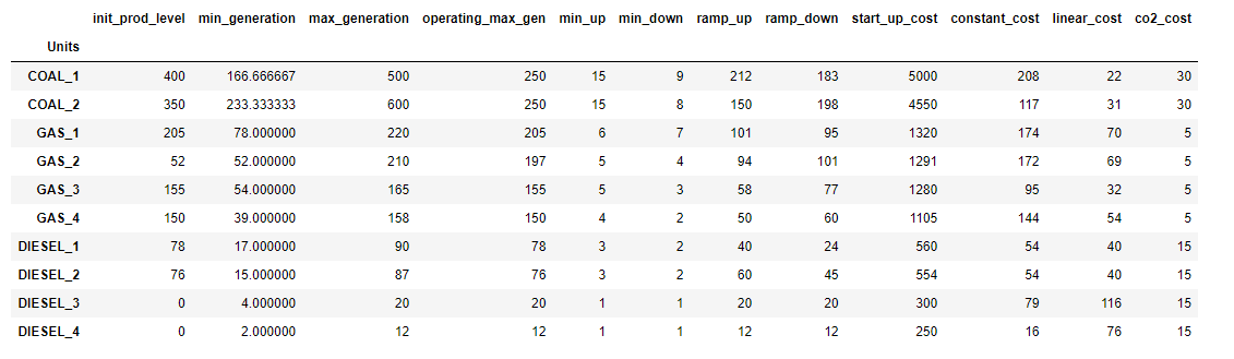
units data frame

The meaning of each of these characteristics is:

• init_prod_level: the initial level of production as the beginning of the planning horizon,
• min_generation and max_generation: the minimum and maximum level of production for this unit,
• operating_max_gen: not used in this problem,
• min_up: the minimum number of periods a unit must be in use after it is switched on,
• min_down: the minimum number of periods a unit must be unused after it is switched off,
• ramp_up and ramp_down: the maximum amount of generation a unit can increase or decrease from one period to the next,
• start_up_cost: the fixed cost to start the unit,
• constant_cost: the fixed cost per period to operate the unit,
• linear_cost: the variable cost per period to produce one unit of energy.
• co2_cost: the variavble ecological cost per period to produce one unit of energy. We see this value changes depending on whether the unit is gas, coal or diesel.

The other important input data frame is pretty simple and represents the load to be covered for each period.

Optimization model

Creating a new empty model is as simple as:

from docplex.mp.model import Model

ucpm = Model("ucp")

Decision variables

The creation of the decision variables is pretty simple using docplex APIs.

The in_use and turn_on variables are binary variables as units, at each period, are either on or off, and either switched on or not, while the production variable is a continuous variable as production can take any value between 0 and a maximum production capacity.

The exchange decision variables define how much electricity is exchanged at a given period.

# in use[u,t] is true iff unit u is in production at period t
in_use = ucpm.binary_var_matrix(keys1=units, keys2=periods, name="in_use")

# true if unit u is turned on at period t
turn_on = ucpm.binary_var_matrix(keys1=units, keys2=periods, name="turn_on")

# true if unit u is switched off at period t
turn_off = ucpm.binary_var_matrix(keys1=units, keys2=periods, name="turn_off")

# production of energy for unit u at period t
production = ucpm.continuous_var_matrix(keys1=units, keys2=periods, name="production")

# exchange of energy at period t
exchange = ucpm.continuous_var_dict(keys=periods, name="exchange")

Constraints

There are many constraints in this pretty realistic model. Let’s just mention and explain a few of these. You can find the complete model in a github repository.

The most important constraint is certainly the one that ensures that for each period, the sum of the production of each unit added to the exchanged quantity must cover the demand. It is pretty simple to formulate. IN our model we use some additional constant robust amount of electricity to make the solution more robust.

for p in periods:
    total_demand = df_loads.value[p]
    ctname = "ct_meet_demand_" + p
    ucpm.add_constraint(ucpm.sum(production[u,p] for u in units) + exchange[p] >= total_demand + robust, ctname)

The constraints to limit how much a unit can increase or decrease the level of production (known as ramp up and ramp down) are a bit more complex, and the first and last period special cases have to be taken into account.

for unit in units:
    u_ramp_up = df_units.value[unit,"ramp_up"]
    u_ramp_down = df_units.value[unit,"ramp_down"]
    u_initial = df_units.value[unit,"init_prod_level"] if (unit,"init_prod_level") in df_units.index else 0
    # Initial ramp up/down
    ucpm.add_constraint(production[unit, firstPeriod] - u_initial <= u_ramp_up)
    ucpm.add_constraint(u_initial - production[unit, firstPeriod] <= u_ramp_down)
    for p in periods:
        if p is not lastPeriod:
            ucpm.add_constraint(production[unit, nextPeriod[p]] - production[unit, p] <= u_ramp_up)
            ucpm.add_constraint(production[unit, p] - production[unit, nextPeriod[p]] <= u_ramp_down)

Some constraints have no direct correspondance to business constraint, but are here to structurally connect some decision variables with some others, such as between turn_off, turn_on and in_use. A bit of logical thinking is required to write these relations as a linear inequations.

for u in units:
    for p in periods:
        if p is not lastPeriod:
            # if unit is off at time t and on at time t+1, then it was turned on at time t+1
            ucpm.add_constraint(in_use[u, nextPeriod[p]] - in_use[u, p] <= turn_on[u, nextPeriod[p]])

            # if unit is on at time t and time t+1, then it was not turned on at time t+1
            # was commented
            ucpm.add_constraint(in_use[u, nextPeriod[p]] + in_use[u, p] + turn_on[u, nextPeriod[p]] <= 2)

            # if unit is on at time t and off at time t+1, then it was turned off at time t+1
            ucpm.add_constraint(in_use[u, p] - in_use[u, nextPeriod[p]] + turn_on[u, nextPeriod[p]] == turn_off[u, nextPeriod[p]])

Then these variables can be linked to the production (no production when unit is off, etc):

# When in use, the production level is constrained to be between min and max generation.
ucpm.add_constraints( production[u,p] <= df_units.value[u,"max_generation"] * in_use[u,p] for u in units for p in periods)
ucpm.add_constraints( production[u,p] >= df_units.value[u,"min_generation"] * in_use[u,p] for u in units for p in periods)

In the model are included other additional constraints.

Objectives

The different costs are easily formulated as expressions of the decision variables.

total_fixed_cost = ucpm.sum(in_use[u,p] * df_units.value[u,"constant_cost"] for u in units for p in periods)

total_variable_cost = ucpm.sum(production[u,p] * df_units.value[u,"linear_cost"] for u in units for p in periods)

total_startup_cost = ucpm.sum(turn_on[u,p] * df_units.value[u,"start_up_cost"] for u in units for p in periods)

total_co2_cost = ucpm.sum(production[u,p] * df_units.value[u,"co2_cost"] for u in units for p in periods)

total_exchange_cost = ucpm.sum(exchange[p] * (df_exchanges.Price[p] if (p) in df_exchanges.index else 0) for p in periods)

Some of these can even be defined as KPIs so that they will be available to be monitored easily from the business application during the solution search.

ucpm.add_kpi(total_fixed_cost   , "Total Fixed Cost")
ucpm.add_kpi(total_variable_cost, "Total Variable Cost")
ucpm.add_kpi(total_startup_cost , "Total Startup Cost")
ucpm.add_kpi(total_economic_cost, "Total Economic Cost")

The objective is to minimize a combination of the five different costs weighted with some coefficients that can be adjusted by the business user to do different what-if analysis.

ucpm.minimize(
    wtotal_fixed_cost * total_fixed_cost 
  + wtotal_variable_cost * total_variable_cost 
  + wtotal_startup_cost * total_startup_cost 
  + wtotal_co2_cost * total_co2_cost 
  + wtotal_exchange_cost * total_exchange_cost)

Solving the problem

After the input data is loaded, the decision variables, constraints and objective formulated, a call to cplex.solve() will look for a solution.

Below is reproduced the log of an execution on my laptop. You can see that with the simple data set, the search for the optimal solution is extremely fast.

Version identifier: 12.10.0.0 | 2019-11-26 | 843d4de2ae
CPXPARAM_Read_DataCheck                          1
CPXPARAM_RandomSeed                              201903125
Tried aggregator 2 times.
MIP Presolve eliminated 3584 rows and 553 columns.
MIP Presolve modified 1480 coefficients.
Aggregator did 9 substitutions.
Reduced MIP has 11756 rows, 6326 columns, and 36950 nonzeros.
Reduced MIP has 4478 binaries, 0 generals, 0 SOSs, and 0 indicators.
Presolve time = 0.05 sec. (36.61 ticks)
Found incumbent of value 1.3770667e+07 after 0.08 sec. (54.65 ticks)
Probing fixed 15 vars, tightened 0 bounds.
Probing changed sense of 5 constraints.
Probing time = 0.05 sec. (9.69 ticks)
Tried aggregator 1 time.
Detecting symmetries...
MIP Presolve eliminated 18 rows and 15 columns.
Reduced MIP has 11738 rows, 6311 columns, and 36804 nonzeros.
Reduced MIP has 4463 binaries, 0 generals, 0 SOSs, and 0 indicators.
Presolve time = 0.05 sec. (24.50 ticks)
Probing time = 0.02 sec. (3.92 ticks)
Clique table members: 20364.
MIP emphasis: balance optimality and feasibility.
MIP search method: dynamic search.
Parallel mode: deterministic, using up to 8 threads.
Root relaxation solution time = 0.05 sec. (21.77 ticks)

Nodes                                         Cuts/
   Node  Left     Objective  IInf  Best Integer    Best Bound    ItCnt     Gap

*     0+    0                       1.37707e+07  2466119.6663            82.09%
*     0     0      integral     0   1.21062e+07   1.21062e+07     1011    0.00%
Elapsed time = 0.28 sec. (140.44 ticks, tree = 0.00 MB, solutions = 2)

Root node processing (before b&c):
  Real time             =    0.30 sec. (140.89 ticks)
Parallel b&c, 8 threads:
  Real time             =    0.00 sec. (0.00 ticks)
  Sync time (average)   =    0.00 sec.
  Wait time (average)   =    0.00 sec.
                          ------------
Total (root+branch&cut) =    0.30 sec. (140.89 ticks)
  Feasible 12106210.666665498

Solution

Some Pandas data frames are created to export the solution, accessing the solution value of the different decision variables.

df_production = pd.DataFrame(columns=['Units', 'Periods', scenario], data=[[u,p,production[u,p].solution_value] for u in units for p in periods])

And the solution can be displayed to the business user.

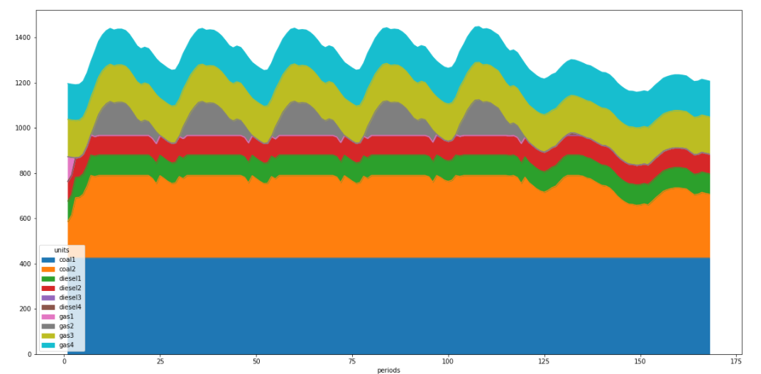
After the model has been developed, debugged, tuned and validated, it can be deployed in production environment and integrated in operational or strategic business solutions.

Here is an example of real execution plan as provided by Red Electrica de España.

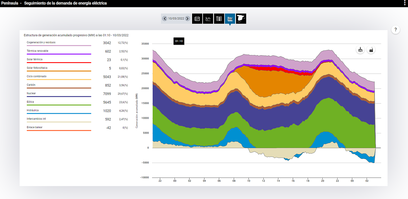
Unit Commitment at Red Electrica de España

As mentioned before, this example is used to demonstrate the ease of integration of Decision Optimization with Planning Analytics.

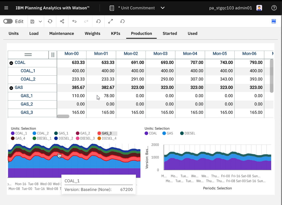
Integration in Planning Analytics

Conclusions

As always with optimization, such models can be used operationally, integrated into a flow for automatic execution in order to take short term decisions with now or low human intervention, or used strategically, doing what-if analysis to support human take longer term decisions, such as the addition of new generation units.

You can find the model and data in this github repository.

For more stories about AI and Business Analytics, follow me on Medium, Twitter or LinkedIn.

[embed]Alain Chabrier - Business Analytics AI STSM - IBM | LinkedIn My expertise is about managing development of software to take better decisions. I have been driving the redesign of…www.linkedin.com