Implementing Sigmoid Activation Function in Hardware
In the world of machine learning, activation functions are the secret sauce that allows neural networks to learn complex, non-linear…
Implementing Sigmoid Activation Function in Hardware
In the world of machine learning, activation functions are the secret sauce that allows neural networks to learn complex, non-linear patterns. Functions like ReLU, Tanh, and the classic sigmoid are fundamental building blocks.

How does sigmoid looks like ?

In Python, implementing one is trivial:
import numpy as np
def sigmoid(x: np.ndarray) -> np.ndarray:
    return 1/(1+np.exp(-x))
input_array=np.array([ -10, -9, -8, -7, -6, -5, -4, -3, -2, -1, 0, 1, 2, 3, 4, 5, 6, 7, 8, 9, 10, 1e6])
output_array=sigmoid(input_array)
print(f"Input array: {input_array}")
print(f"Output array after Sigmoid: {output_array}")
sigmoid function

Derivatives of the sigmoid function and its PLAN approximation
Method of Approximating sigmoid Activation function for Hardware
In this article, Will use two key techniques: Piecewise Linear (PLAN) Approximation and Fixed-Point Arithmetic.Below Research Paper has explored the implementation in much detail .

What makes it difficult to model in hardware?
Exponentiation (e⁻ˣ): There is no exp() logic gate. Calculating an exponent requires complex, iterative algorithms (like CORDIC) or massive, pre-calculated lookup tables (LUTs). Both are slow and resource-hungry.
Division: Like exponents, division isn’t a single-clock-cycle operation. It requires a sequential algorithm that takes many cycles to complete, creating a bottleneck in our data pipeline.
The core idea of PLAN is simple: if a smooth curve is too hard to build, let’s approximate it with a few simple, connected straight lines.
A straight line is defined by the equation:
y = mx + c
This only requires (one multiplication and one addition) operations that are much more manageable in hardware. By defining several different line segments for different input ranges, we can create a shape that is “good enough” to replace the real sigmoid curve without sacrificing too much accuracy.
For the approximation :

And for negative values, we use the following property:

Fixed-Point Arithmetic
Equations are great, but they still contain decimal (floating-point) numbers, which we want to avoid as we have to use Floating point unit for that . The next step is to convert this entire system to use only integers, using a technique called fixed-point arithmetic.
The idea is to pre-multiply all our numbers by a scaling factor. A common choice is a power of two 2¹⁶ (65536).
Real numbers are converted to integers and cut off the fractional part By doing this, we can represent fractional numbers with integers, with an implicit understanding of where the “binary point” is.
when we look at our multipliers
- 0.25 is 1/4 -> a right bit-shift by 2 (>> 2)
- 0.125 is 1/8 -> a right bit-shift by 3 (>> 3)
- 0.03125 is 1/32 -> a right bit-shift by 5 (>> 5)
Have just replaced expensive multiplications with virtually free bit-shifts! So the equations will become

For the implementation of the expression on the FPGA no multipliers are needed, it is enough to use shifting registers and adders.
Hardware Implementation
This Parametrizable module implements our final integer-only algorithm in System Verilog.
`timescale 1ns/1ps
module sigmoid #(
    parameter DATA_WIDTH = 32
)(
    input  logic signed [DATA_WIDTH-1:0] i_data,
    output logic signed [DATA_WIDTH-1:0] o_data
);
    localparam signed [DATA_WIDTH-1:0] THRESHOLD_5_0   = 32'sd327680; // 5.0 * 65536
    localparam signed [DATA_WIDTH-1:0] THRESHOLD_2_375 = 32'sd155648; // 2.375 * 65536
    localparam signed [DATA_WIDTH-1:0] THRESHOLD_1_0   = 32'sd65536;  // 1.0 * 65536
    localparam signed [DATA_WIDTH-1:0] OFFSET_A        = 32'sd55296;  // 0.84375 * 65536
    localparam signed [DATA_WIDTH-1:0] OFFSET_B        = 32'sd40960;  // 0.625 * 65536
    localparam signed [DATA_WIDTH-1:0] OFFSET_C        = 32'sd32768;  // 0.5 * 65536
    localparam signed [DATA_WIDTH-1:0] ONE_VAL         = 32'sd65536;  // 1.0 * 65536

    logic signed [DATA_WIDTH-1:0] abs_data;
    logic                         is_negative;
    logic signed [DATA_WIDTH-1:0] pwl_result;

    always_comb begin
        is_negative = i_data[DATA_WIDTH-1];
        if (is_negative) begin
            abs_data = -i_data;
        end else begin
            abs_data = i_data;
        end

        if (abs_data >= THRESHOLD_5_0) begin
            pwl_result = ONE_VAL;
        end
        else if (abs_data >= THRESHOLD_2_375) begin
            pwl_result = (abs_data >>> 5) + OFFSET_A;
        end
        else if (abs_data >= THRESHOLD_1_0) begin
            pwl_result = (abs_data >>> 3) + OFFSET_B;
        end
        else begin
            pwl_result = (abs_data >>> 2) + OFFSET_C;
        end

        // if negative values appear use: f(-x) = 1 - f(x)
        if (is_negative) begin
            o_data = ONE_VAL - pwl_result;
        end else begin
            o_data = pwl_result;
        end
    end

endmodule
Verification with a Python Testbench (Cocotb)
How do we know it works? We test it against our original NumPy model! Using the Cocotb framework, we can write a Python testbench to feed in vectors and verify the hardware’s output is close enough to the “golden” software version.
import cocotb
from cocotb.triggers import Timer
import numpy as np

# Golden Software Model and Test Vectors
def sigmoid_sw(x: np.ndarray) -> np.ndarray:
    return 1 / (1 + np.exp(-x))

INPUT_VECTORS_FLOAT = np.array([
    -10, -9, -8, -7, -6, -5, -4, -3, -2, -1, 0,
    1, 2, 3, 4, 5, 6, 7, 8, 9, 10
])

SCALE = 65536  # 2^16

def float_to_fixed(value):
    return int(round(value * SCALE))

def fixed_to_float(value):
    return float(value) / SCALE

#Cocotb TestBench
@cocotb.test()
async def sigmoid_32bit_vector_test(dut):
    expected_results_float = sigmoid_sw(INPUT_VECTORS_FLOAT)
    tolerance = 0.02

    for input_float, expected_float in zip(INPUT_VECTORS_FLOAT, expected_results_float):
        dut._log.info(f"Testing input value: {input_float}")
        input_fixed = float_to_fixed(input_float)
        dut.i_data.value = input_fixed
        await Timer(1, units="ns")

        hw_output_fixed = dut.o_data.value.signed_integer
        hw_output_float = fixed_to_float(hw_output_fixed)

        error = abs(hw_output_float - expected_float)

        dut._log.info(f"Input(float): {input_float:<7.2f} -> HW Output(float): {hw_output_float:.6f}")
        dut._log.info(f"SW Expected(float): {expected_float:.6f} -> Error: {error:.6f}")

        assert error < tolerance, \
            f"FAIL! Input {input_float} -> Error {error} exceeds tolerance {tolerance}."

        dut._log.info("PASS: Hardware output is within tolerance.")

    dut._log.info("SUCCESS")
Running the test confirms that our hardware approximation works, with a maximum error of less than 2%, which is fantastic for most neural network applications.

Running test cases and passing 😎
By trading a small amount of mathematical precision for a huge gain in speed and resource efficiency, we can build hardware that performs inference orders of magnitude faster than a CPU.
A Parting Thought: Why We Don’t Always Use sigmoid Anymore
You might have noticed that modern networks often prefer ReLU. That’s because sigmoid suffers from the “vanishing gradient problem.” For very large or very small inputs, the slope of the sigmoid curve becomes nearly zero. During training, this can cause the learning process to slow down or stop entirely for deep networks. Still, sigmoid is useful in output layers (probabilities)

Thanks for reading! If you found this useful, feel free to connect on LinkedIn or leave a comment below.Follow for more Cooooool hardware content!!
Reference
메타데이터
- post_id
- cdab8e1bd9a9
- slug
- implementing-sigmoid-activation-function-in-hardware-cdab8e1bd9a9
- url
- https://blog.devgenius.io/implementing-sigmoid-activation-function-in-hardware-cdab8e1bd9a9
- canonical_url
- https://blog.devgenius.io/implementing-sigmoid-activation-function-in-hardware-cdab8e1bd9a9
- author_url
- https://medium.com/@ayushdixithere
- status
- ok
- fetched_at
- 2026-08-05 03:43:09