Identifying fiscal consolidation episodes in OECD countries using the CUSUM method

**Disclaimer:** This is a working draft, i.e., research in progress and is such, published to elicit comments/advice/recommendations and to encourage debate. The views expressed in this article are solely mine.

Summary: I explore whether I can use the Cumulative Sum (CUSUM) change-point detection algorithm to accurately identify fiscal consolidation episodes across cyclically adjusted primary balance (CAPB) data for around 80 IMF countries between the 1990s to 2022. Results show that CUSUM has about 67.18% overall accuracy in correctly identifying fiscal consolidation episodes, with a 95% confidence interval of 61.79% to 72.25%. Moreover, sensitivity, or true positive rate (proportion of correctly predicted fiscal consolidation episodes), is 81.56% and specificity, or true negative rate (proportion of episodes without any fiscal consolidation episodes), is 0.4966. Effectively, using CUSUM on CAPB data is better at identifying a fiscal consolidation episode than identifying when it is NOT a fiscal consolidation episode.

Introduction & some definitions

Typically, it’s tricky to identify fiscal consolidation episodes for many countries. A qualitative research approach, often called the “narrative” approach, would likely be better. A prime example for the narrative approach is the work done by Alesina, et al. In the 2020 “Austerity: When It Works and When it Doesn’t” book by Alberto Alesina, Carlo Favero, and Francesco Giavazzi, one of the main contributions to the literature is a panel dataset of close to 200 austerity plans in 16 high-income OECD countries from the late 1970s until 2014. The dataset documents exogenous shifts in fiscal variables categorized between direct and indirect taxes, transfers, and other government spending reconstructed from original documents concerning about 3,500 individual fiscal measures. However, documenting austerity plans from primary documentation requires substantial resources and time.

In this short note, I propose the application of the classic CUSUM (cumulative sum) change-point detection algorithm, commonly used in sequential analysis, to automatically identify episodes of fiscal consolidation across 80 IMF countries between the 1990s to 2022. Specifically, I explore whether CUSUM can identify periods of fiscal consolidation when applied to the IMF Fiscal Monitor’s cyclically adjusted primary balance (% of potential GDP) or CAPB. The CUSUM algorithm is a sequential analysis technique typically used in quality control for production processes and change-point detection. The CUSUM technique allows users to flexibly identify cumulative sum change in a variable, in this case, CAPB. CUSUM provides rapid analysis and identification of trends in a data series, with a simple framework. The assumption here is that sequential and cumulative CAPB surpluses can be an indicator to identify episodes of fiscal consolidation. Moreover, I assume that one positive delta CAPB value is inadequate to determine fiscal consolidation episodes. Instead, sequential positive % changes in CAPB are an approximate condition. In practice, this is somewhat of a reasonable assumption. In general, most countries implement fiscal consolidation strategies over the medium term.

The OECD, among other international institutions, defines fiscal consolidations mainly along the following lines: concrete policies aimed at reducing government deficits and debt accumulation. Fiscal consolidation measures are often structural but may not be so; they may include pension accounting changes, one-off or temporary measures and rolling back stimulus measures. Economic growth can also reduce primary balance deficits, leading to more revenues and less expenditure, e.g. , unemployment, when more people find jobs (cyclical effects). To disentangle the cyclical effects of fiscal consolidation policies on the primary balance, I use the cyclically adjusted primary balance.

Section I: Identifying periods of fiscal consolidation

Data Import & Process

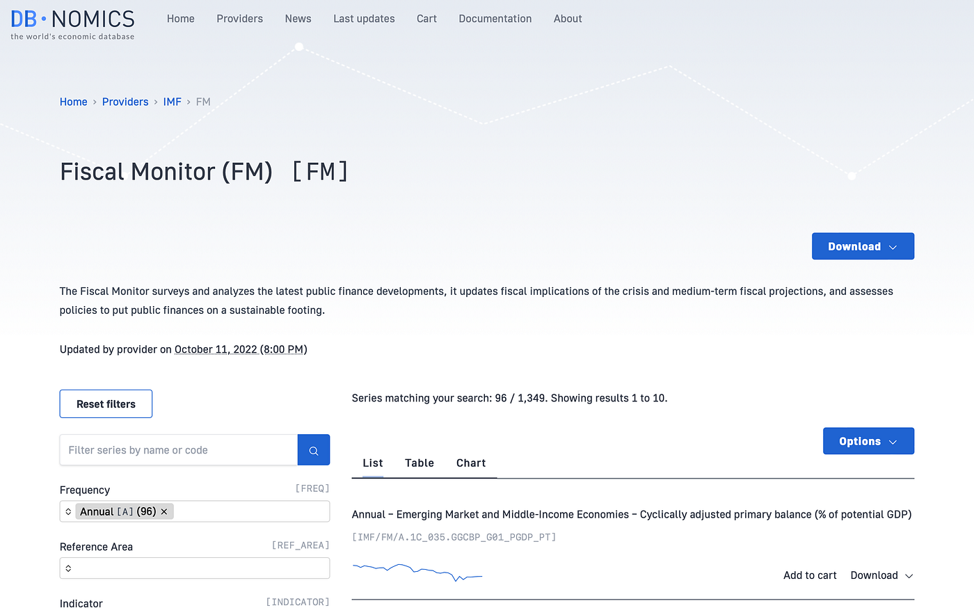
The Fiscal Monitor CAPB variable is imported through the DBnomics R package to conduct the analysis. DBnomics is a fantastic repository of economic data from different providers (national and international statistical institutes, central banks, etc.), for free (db.nomics.world), while the R package allows users to interact and download data through the API.

Data Exploration using Italy

Once the data are downloaded, we look at the raw CAPB variable for Italy to get a sense behind the data. Here, we print several observations of the data for Italy, where capb is cyclically adjusted primary balance, delta_capb is change in cyclically adjusted primary balance (i.e., delta_capb = CAPB_t -CAPB_t-1), and delta_capb_pct is the percent change in cyclically adjusted primary balance (i.e., delta_capb = (CAPB_t -CAPB_t-1)/CAPB_t-1 100*).

Similarly, the variables cusum_mu and cusum_sd are pooled sample mean and standard deviation, respectively.

Fig. 1a and Fig. 1b show the time-series data for Italy. In Fig. 1a CAPB drastically increases throughout the 1990s, indicating large government surpluses, and then somewhat in the late 2000s. Italy’s CAPB plummets to -2.5 in 2020 as it faces large budgetary deficits and a Eurozone sovereign debt crisis. Similarly in Fig. 1b, the single most significant decrease in CAPB is in 2020, likely indicating the effect of the ongoing COVID-19 pandemic. Fig. 1b shows that the majority of CAPB changes lie between the bounds of -2 and 2 percent of potential GDP. This suggests changes in Italy’s CAPB larger than 2 percent of potential GDP is a large budgetary change, particularly year on year.

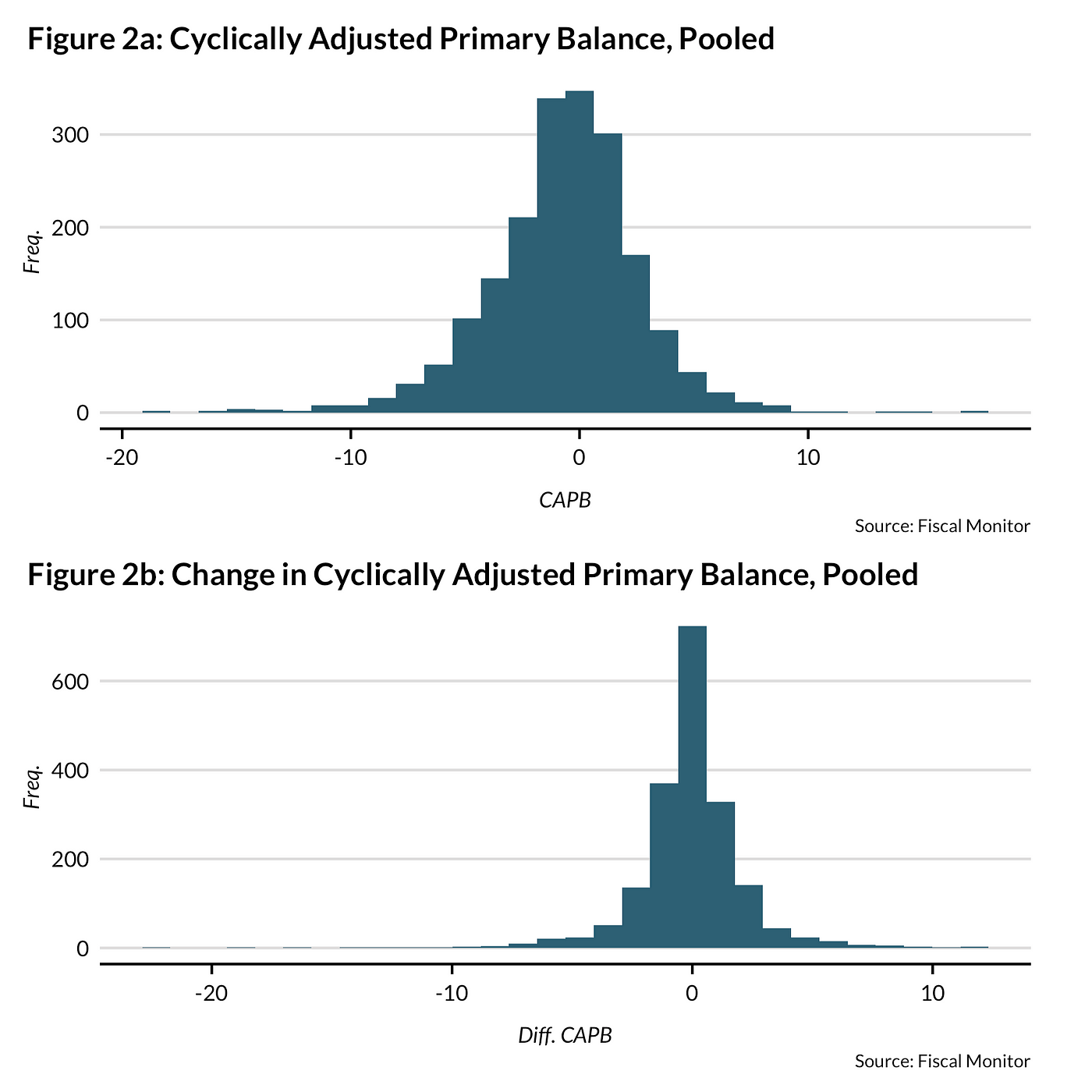
For a bigger picture, I examined the distribution of the complete pooled data with two histograms. Both CAPB and delta CAPB have distributions remarkably close to a normal distribution, albeit with skew on the left tail. In particular, Fig. 2b implies that the overwhelming majority of changes in CAPB are within -10 to 10 percent of potential GDP year on year. As a side note, the normal distribution of the CAPB and delta CAPB variable suggests it may be suitable for efficient estimators in the least squares analysis.

Methodology: CUSUM

The CUSUM technique involves the calculation of a cumulative sum (which is what makes it “sequential”). The general model for CUSUM is the following: S_t= max(0, S_t-1 + x_t - mu_t), where x_t is the observed value at time t, mu_t is the expected value of x_t if there are no changes, and S_t is the metric. The basic idea is to declare an observed change when and if the metric S_t goes above a threshold T. Note the above formula only detects changes in the positive direction.

At each time period, we observe x_t see how much more it is above the expectation. Then, we add the value to the previous metric S_t-1, to give the running total S_t. If that running total S_t is greater than zero, we keep it, but if it’s less than zero, we reset the running total to zero. This helps CUSUM detect changes quickly. Note that the initial value of the metric is set as S_0 = 0. Effectively, the main goal of a control chart is to monitor a process. If special causes of variation are present, the process is said to be “out of control” and flagged by the CUSUM technique. A process is declared to be “in control” if all points charted lie randomly within the control limits..

The variable x_t that we use is the change in cyclically adjusted primary balance i.e., delta_CAPB = CAPB_t — CAPB_t-1. Recall that the formula for CAPB is CAPB = R(Yp/Y)^ε_R — G(Yp/Y)^ε_G, where R is nominal primary revenue, Yp is potential output (that is, the maximum output compatible, at any given time, with the absence of unexpected inflation), Y is actual output and ε is elasticity of revenue or expenditure with respect to the output gap.

Ideally, the CUSUM statistic S_t should remain smaller than the threshold if a fiscal consolidation is not occurring and quickly cross the threshold if a fiscal consolidation episode occurs. In some uses of CUSUM, a typical choice for threshold T is 5 standard deviations, while C will be half of a standard deviation. But in the case of cyclically adjusted primary balance, those “standard” thresholds are probably too conservative. Therefore, the values of both T and C are set far lower (and can be calibrated based on previous data) than the typical threshold. When the change in CAPB changes positively, CUSUM should be able to detect the change quickly and identify the fiscal consolidation episode.

Example case study: Italy

I first show an example of Italy. Note the CUSUM parameters: mu_t is the central line, and the argument decision.int is the numeric value specifying the number of standard errors of the summary statistics at which the cumulative sum is out of control, i.e., threshold T. Finally, the amount of shift in the process to be detected by the CUSUM chart, measured in standard errors of the summary statistics, is controlled by the argument se.shift, by default set at 1.

The qcc package automatically plots a Shewhart chart. Note that the control chart has the center line (horizontal solid line), the upper and lower control limits (dashed lines), i.e., threshold T, and sample group statistics, drawn as points connected with lines. The red dots above the UDB are observations flagged as “out of control,” i.e., as episodes of fiscal consolidation. Similarly, the red dots below the LDB may be considered episodes of fiscal expansion. In Italy’s case, the period in the 1990s is flagged as a fiscal consolidation episode, as are 2007 and 2012–2013.

Results of CUSUM approach

Fig. 4 depicts the countries flagged as undergoing a fiscal consolidation episode as a share of total countries in that period. Interestingly, advanced and emerging market economies are in sync — which suggests most countries, as identified by CUSUM, experience fiscal consolidation episodes simultaenously. Distances between the peaks of identified fiscal consolidation episodes (when more than half of countries are flagged) are a little less than 10 years on average.

Going back to our country case study for Italy, the below table presents the first several observations of the final results.

In particular, Fig. 5 depicts CAPB over time, with vertical red lines to show years flagged as a fiscal consolidation episode by CUSUM.

Section II: Evaluating the CUSUM approach

To evaluate whether CUSUM is accurate at identifying fiscal consolidation episodes, I merged the estimations with Alesina’s dataset of fiscal consolidation using the narrative approach. The idea is that Alesina’s narrative approach presents a granular dataset to compare the CUSUM approach to.

The dataset accompanying the book by Alesina, et al includes a dummy variable for fiscal consolidation measures (consolidation dummies a_t+1 & consolidation dummies u_t), and offers an easy way of comparing the CUSUM predictions. The table below shows a glimpse of the dataset made available by Alesina, et al.

Using the confusion matrix function from R’s caret package, I show CUSUM’s performance metrics. Overall accuracy is around 67.18%, with 95% CI of 61.79% to 72.25%. Moreover, sensitivity, or true positive rate (proportion of correctly predicted fiscal consolidation episode), is 81.56% and specificity, or true negative rate (proportion of episodes without any fiscal consolidation episodes), is 0.4966.

This suggests that CUSUM is better at identifying a fiscal consolidation episode, than when it is NOT a fiscal consolidation episode.

In evaluating the CUSUM predictions, a couple of issues come to mind. First, deciding the threshold parameter value for CUSUM requires some trial and error. The typical choice for threshold T is 5 standard deviations, which is far too conservative for CAPB data. The threshold of 0.5 used in this analysis is far lower than the typical choice. Further work may show higher or lower thresholds for out of sample accuracy improvements.

Second, the low specificity (i.e., true negative rate or correctly identifying when there isn’t a fiscal consolidation episodes) is very low at 49.66%. This suggests that for certain countries, using CAPB may result in incorrectly flagging a fiscal consolidation episode, when in fact, there has been no fiscal consolidation policies. Indeed, other factors leading to fiscal surpluses are not specific fiscal consolidation policies. If these other factors are not properly controlled for in regression analytical work, estimates may suffer from endogeneity.

Appendix

Bibliography

• https://www.rdocumentation.org/packages/caret/versions/3.45/topics/confusionMatrix
• https://cran.r-project.org/web/packages/rdbnomics/vignettes/rdbnomics.html#2_Fetch_time_series_by_ids
• https://www.oecd.org/economy/growth/fiscal-consolidation-what-factors-determine-the-success-of-consolidation-efforts.pdf
• http://www.stat.unipg.it/luca/misc/Rnews_2004-1-pag11-17.pdf
• https://www.openicpsr.org/openicpsr/project/114028/version/V1/view
• https://www.aeaweb.org/articles?id=10.1257/jep.33.2.141
• https://www.harvard.com/book/austerity/
• https://cran.r-project.org/web/packages/rdbnomics/rdbnomics.pdf
• https://www.rdocumentation.org/packages/qcc/versions/2.6/topics/cusum
• https://stats.stackexchange.com/questions/168481/how-find-controls-limits-for-cusum-chart
• http://www.cookbook-r.com/Manipulating_data/Renaming_columns_in_a_data_frame/
• https://community.rstudio.com/t/help-how-to-flag-consecutive-non-zero-values/48936/2
• https://rmarkdown.rstudio.com/lesson-5.html
• https://bookdown.org/yihui/rmarkdown-cookbook/chunk-options.html
• https://stackoverflow.com/questions/29648907/using-geom-rect-for-time-series-shading-in-r/29649575
• https://thomasleeper.com/Rcourse/Tutorials/vectorindexing.html
• https://stats.oecd.org/Index.aspx?DataSetCode=SNA_TABLE11
• https://stackoverflow.com/questions/47710427/how-to-show-code-but-hide-output-in-rmarkdown