Understanding UMAP (Uniform Manifold Approximation and Projection)

Revolutionizing Dimensionality Reduction in Machine Learning

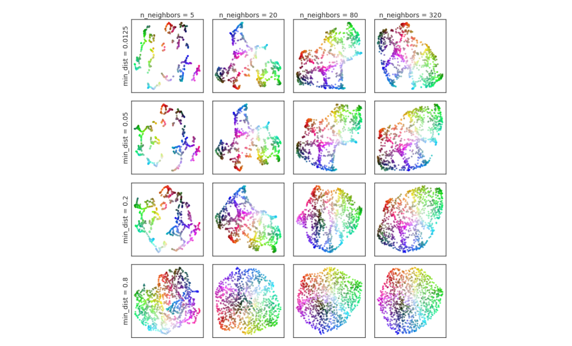
Dimentionality Reduction is an important concept which is very crucial for data analysis and visualization. As the number of features or dimensions in a dataset increases, the amount of data required to generalize them accurately also increases exponentially, and introduces several issues which hinders the performance of machine learning algorithms and make data analysis more challenging. This phenomenon is called curse of dimentionality. Dimensionality reduction methods address this problem by transforming the original high-dimensional feature space into a lower-dimensional representation while preserving essential information. Thus, these techniques not only enhance the computational efficiency of algorithms but also mitigate overfitting, as they help focus on the most relevant features and reduce the impact of noise.

There has been several methods for Dimentionality reduction, based on the implicit technique, they can broadly categorized in two classes:-

1. Linear Dimensionality Reduction Techniques: These techniques are a class of methods employed in data analysis and machine learning that aim to reduce the number of features or dimensions in a dataset while maintaining linearity in the transformation. These techniques operate on the premise that the relationships among the original variables can be effectively captured through linear combinations. Principal Component Analysis (PCA), Linear Discriminant Analysis (LDA), Multidimensional Scaling (MDS), and Singular Value Decomposition (SVD) are common representatives of this class. By identifying and emphasizing the most informative directions or linear combinations of features, linear dimensionality reduction techniques enable the creation of a lower-dimensional representation of the data that retains a significant portion of the original variance. These methods find applications in tasks such as feature selection, visualization, and noise reduction, contributing to improved computational efficiency and interpretability in various analytical and modeling endeavors.
2. Nonlinear Dimensionality Reduction Techniques: Thesse are class of methods used in data analysis and machine learning that aim to reduce the dimensionality of a dataset while accommodating nonlinear relationships among variables. In contrast to linear techniques, these methods acknowledge and capture the complex, non-rectilinear structures present in high-dimensional data. Examples of Nonlinear Dimensionality Reduction Techniques include t-Distributed Stochastic Neighbor Embedding (t-SNE), Isomap (Isometric Mapping), and Autoencoders. These techniques are particularly effective in preserving local and global structures, uncovering intricate patterns, and revealing the underlying intrinsic geometry of the data. By transforming high-dimensional data into lower-dimensional representations that reflect nonlinear relationships, these methods enhance the interpretability of complex datasets, aid in visualization, and contribute to improved performance in tasks such as clustering and classification.

Classical methods like Principal Component Analysis (PCA) and t-distributed Stochastic Neighbor Embedding (t-SNE) have been widely used for dimensionality reduction. However, these techniques have limitations, such as sensitivity to noise or inability to capture complex non-linear relationships in the data. **Uniform Manifold Approximation and Projection (UMAP) {Leland et. al. 2018}, **is a recent development in the area of dimentionality reduction which offers several benefits over traditional methods:

1. Preservation of Nonlinear Relationships: UMAP is particularly adept at capturing nonlinear relationships in data. Traditional linear methods like PCA are limited in their ability to represent complex, nonlinear structures. UMAP’s capacity to preserve both local and global nonlinear relationships makes it more suitable for datasets with intricate patterns.
2. Better Handling of Local Structure: UMAP tends to perform well in preserving the local structure of the data, capturing clusters and groups effectively. This is crucial in situations where preserving the local relationships between data points is essential, such as in clustering or identifying similar items in a dataset.
3. Adaptive Parameterization: UMAP provides more flexibility through adaptive parameterization, allowing users to adjust the trade-off between preserving local and global structures. This adaptability is advantageous when dealing with datasets that exhibit varying degrees of local and global complexity.
4. Robustness to Noise: UMAP has demonstrated robustness to noisy data compared to some traditional methods. It can handle noisy or outlier data points more gracefully, contributing to a more reliable representation of the underlying structure in the presence of noise.
5. Scalability: UMAP is designed to scale well with larger datasets, making it suitable for high-dimensional data with a substantial number of samples. Traditional methods may face challenges in terms of computational efficiency and scalability as the dimensionality and size of the dataset increase.

===============================================================

Now, as I have got you hyped about UMAP, so let’s dig deeper

UMAP, was introduced by Leland McInnes, John Healy, and James Melville in 2018, it gained immediate popularity for its ability to address the shortcomings of traditional methods. UMAP belongs to the family of manifold learning techniques and stands out for its efficiency, scalability, and capability to capture both local and global structures in the data.

Some Key Features of UMAP

1. Preservation of Local and Global Structure: UMAP excels in preserving both local and global relationships within the data. This is crucial for maintaining the integrity of the information, as it ensures that nearby points in the high-dimensional space are still close to each other in the reduced-dimensional space.
2. Efficiency and Scalability: UMAP is known for its computational efficiency, allowing for the analysis of large datasets without sacrificing accuracy. This scalability is particularly valuable in the age of big data, where traditional methods may struggle to handle vast amounts of information.
3. Non-Linearity: Unlike PCA, which assumes linear relationships, UMAP can capture non-linear structures in the data. This makes it suitable for scenarios where the underlying relationships are complex and cannot be adequately represented by linear transformations.
4. Parameter Tuning: UMAP provides users with flexibility through adjustable parameters, allowing for fine-tuning based on the characteristics of the dataset and the desired output. This adaptability enhances the algorithm’s applicability to a wide range of data types.

How UMAP Works?

Uniform Manifold Approximation and Projection (UMAP) involves several mathematical concepts and steps. Lets understand the steps involved first:

Suppose you have a high dimensional dataset with you, in UMAP we start with

STEP 1 Constructing a Graph Representation

Building a High-Dimensional Graph:

• UMAP starts by constructing a high-dimensional graph representation of the data.
• Each data point is considered as a node in the graph, and edges are drawn between points based on their similarity in the high-dimensional space.

Local and Global Relationships:

• UMAP aims to preserve both local and global structures in the data. Local relationships are maintained by connecting each point to its nearest neighbors.
• Global relationships are captured through connectivity patterns that extend beyond immediate neighbors.

STEP 2 Fuzzy-Simplicial Set Approximation

Fuzzy-Simplicial Set:

• UMAP represents the graph as a fuzzy-simplicial set, which allows for the inclusion of uncertainty in the relationships between points.
• A simplicial set is a mathematical structure that encodes the relationships between different subsets of points.

Optimizing a Low-Dimensional Representation:

• UMAP then aims to find a low-dimensional representation that approximates the fuzzy-simplicial set in a way that preserves the local and global relationships present in the high-dimensional space.
• The optimization process involves minimizing a cost function that penalizes discrepancies between the high-dimensional and low-dimensional representations.

STEP 3 SGD Optimization:

Optimization Algorithm:

• UMAP uses stochastic gradient descent (SGD) to optimize the low-dimensional representation.
• SGD is an iterative optimization algorithm that adjusts the positions of points in the low-dimensional space to minimize the cost function.

Balancing Attraction and Repulsion:

• UMAP incorporates both attractive and repulsive forces during the optimization process. Points that are similar in the high-dimensional space are attracted to each other in the low-dimensional space, while dissimilar points are pushed apart.

STEP 4 Resulting Low-Dimensional Representation

• Final Embedding:
• After the optimization process, UMAP provides a low-dimensional representation of the data, typically in two or three dimensions.
• This representation captures the essential structures and relationships present in the high-dimensional space.

Did you get the intuition behind the UMAP?

Now, lets understand it using mathematical theory behind it:-

Assume we have a high-dimensional dataset with N data points, each having D features. Let’s represent this dataset as X with dimensions N×D.

For each data point x_i​ in X, find its k nearest neighbors based on a distance metric (e.g., Euclidean distance). This forms the initial graph structure.

Neighbors(x_i)={x_j,x_k,…}

for i=1,2,…,N

Next, define a fuzzy-simplicial set S that captures the local and global relationships in the dataset. This involves assigning membership values fuzzy_sim(x_i,x_j) to represent the strength of the relationship between points x_i and x_j​.

here:

• D(x_i, x_j) is the Euclidean distance between x_i and x_j​,
• σ_i and σ_j are local scaling parameters for points x_i and x_j​, respectively.

For each pair of neighbors (x_i, x_j), calculate fuzzy_sim(x_i, x_j). This forms a high-dimensional fuzzy-simplicial set S. This fuzzy-simplicial set construction introduces the concept of a local neighborhood around each point.

Next, define a cost function that measures the difference between the high-dimensional fuzzy-simplicial set S and its low-dimensional counterpart S′.

UMAP uses cross-entropy as the cost function:

Here:

• y_i​ and y_j​ are the low-dimensional representations of x_i​ and x_j​,
• fuzzy_sim′ represents the low-dimensional fuzzy-simplicial set.

Next, Update the low-dimensional representations by minimization of cost function using stochastic gradient descent:

Here

• ​y_i ^(t) is the low-dimensional representation of x_i​ at iteration t,
• η is the learning rate, repeat until converge.

After optimization, y_i values represent the low-dimensional embeddings of the N data points. These values typically provide a 2D or 3D representation of the data that preserves its essential structures.

Applications of UMAP

UMAP has been applied in various fields, including genomics, where it has helped reveal cryptic population structures and phenotype correlations. It has also been used to discover fine-scale relationships between geography, genotypes, and phenotypes in population datasets.

Apart from Genomics, it has been applied to several area where we have to encounter curse of dimentionality:

Classical Machine Learning: UMAP is employed in various machine learning tasks, such as clustering, classification, and anomaly detection. Its ability to preserve the intrinsic structure of the data makes it a valuable preprocessing step for improving the performance of machine learning models.

Image Analysis: UMAP has proven effective in image analysis, aiding researchers and practitioners in visualizing and exploring high-dimensional image datasets. This is particularly valuable in fields such as computer vision and medical imaging.

Social Network Analysis: UMAP is applied to understand and visualize relationships in social networks. By reducing the dimensionality of the data while preserving relevant structures, it becomes easier to identify communities and patterns in large-scale social graphs.

===============================================================

In summary, UMAP stands out as a crucial tool for exploratory data analysis and preprocessing within machine learning pipelines, thanks to its efficient handling of large datasets and its adept preservation of both local and global data structures.

For individuals seeking a more in-depth understanding of UMAP, the original paper and subsequent tutorials offer a comprehensive exploration of the algorithm and its diverse applications. Please note, that UMAP is an area of active research, with continuous developments aimed at enhancing its capabilities and discovering new avenues of application. UMAP’s primary drawback lies in its lack of maturity. As a relatively new technique, the associated libraries and best practices are not firmly established or robust. Nevertheless, for those who are open to being early adopters, UMAP presents considerable potential and benefits.

Resources : paper , Python package.