An Introduction to Algorithms, Pt. 3: Efficiency && Big-O Time Complexity

Now that you’re familiar with sequencing, selection, and iteration, it’s time to take your understanding of algorithms to the next level by exploring the idea that not all algorithms are created equal. Some complete their task in a matter of microseconds, while others seem to drag on forever. In this article, you’ll learn about Big-O notation and the difference between reasonable and unreasonable runtime. You’ll also take your first steps towards assessing relative efficiency with an example: linear search versus binary search. This knowledge will lead you to write more efficient algorithms that will set you apart as a developer.

Big-O Notation (n.) a formal expression of an algorithm’s complexity in relation to the growth of the input size. It is used to rank algorithms based on their performance with large inputs.

Reasonable vs. Unreasonable Runtime

Runtime is the execution time of an algorithm. In other words, the amount of time it takes to complete its intended task. We can break it into two distinct performance classes.

1. Reasonable (a.k.a., “polynomial”) time describes any runtime that does not increase faster than n^k. Examples include: constant time (n^0), logarithmic time (log n), linear time (n), and quadratic time (n^2)
2. Unreasonable (a.k.a., “superpolynomial”) time describes any runtime that increases faster than n^k. Examples include: exponential time (2^n) and factorial time (n!)

The ability to scale effectively with the size of a given input determines this distinction between reasonable and unreasonable. Algorithms with reasonable runtime have predictable, limited growth in execution time as input size increases. On the other hand, algorithms with unreasonable runtime have exponential or even faster growth in execution time as input size increases. It’s crucial to understand the complexities of the algorithm(s) that you’re working with and to strive for reasonable runtime whenever possible so that your programs perform well and scale effectively.

Now, let’s take a closer look at how some of the most common Big-O runtimes compare in terms of their scaling behavior.

This chart goes beyond reasonable and unreasonable. It analyzes seven different runtimes and rates them from “horrible” to “excellent”. Note that quadratic time — O(n²) — is “horrible” despite its reasonable status in traditional computer science circles. This example indicates that there are levels to time complexity analysis and that even if your algorithm is reasonable, there may still be room for improvement and optimization.

Linear vs. Binary Search

a linear search algorithm in JavaScript

Linear search algorithms run in linear Big-O time: O(n). Their execution time is directly proportional to the size of the data set they’re searching.

Imagine you have a list of 100 numbers and a linear search algorithm to help you find the one you want. Unfortunately, it’s at the end of the list. So if it takes one millisecond for your algorithm to evaluate a number and determine whether it’s the one you want, you will have to wait 100ms. If you think about it, 100ms is only 1/10 of a second. So your algorithm is fast. Right? Wrong.

Replace your 100-number data set with 1,000,000 numbers. Now how long will you have to wait? Worst-case 1,000,000ms, which is more than 16 minutes. Now we have a problem. The good news is that we also have a solution in binary search.

a binary search algorithm in JavaScript

Binary search algorithms run in logarithmic Big-O time: O(log n), which is exceptionally fast. The catch is that they only work on sorted lists. If you read the code carefully, you’ll see that they work by establishing (and recursively updating) a low-index and a high-index in a given array. They find the element halfway between those indices and check to see if it matches the target. If it does, they return the index position of the target. Otherwise, they update the appropriate index and repeat the process.

This method is remarkably similar to searching for the word iteration in a physical dictionary with 960 pages. You would first open it to one of the middle pages and evaluate the words. If they follow iteration alphabetically (i.e., they all start with the letter “m”), you know that your target word is in the first half of the dictionary. So, instead of searching through 960 pages, you are only dealing with 480. Remarkable! Now, repeat this process until you find the word iteration. This method is a brilliant example of logarithmic time complexity because the amount of time it takes to find the word increases logarithmically with the number of pages in your dictionary.

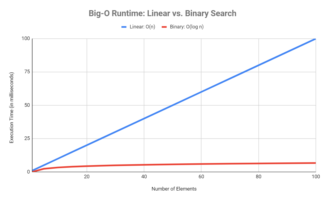
This graph depicts the worst-case execution time of linear and binary search algorithms, assuming (arbitrarily) that it takes 1ms to evaluate each element.

If you look closely at the graph, it’s clear that the binary search algorithm is significantly more efficient — even when dealing with a data set that only contains 100 elements. But what if we were dealing with a data set of 1,000,000 elements? Remember that (worst-case) a linear algorithm takes ~16 minutes to find its target. On the other hand, a binary search algorithm will only take 19.93 milliseconds. That’s an extraordinary difference! Let’s run one final scenario with 1,000,000,000 (one billion) elements. Working with this massive data set, a linear search algorithm would take more than 11 days to find its target, but a binary search algorithm would only take ~29.90 milliseconds. Unbelievable. This extreme disparity is why it’s so important to write efficient algorithms.

This chart depicts the worst-case execution time of linear and binary search algorithms, assuming (arbitrarily) that it takes 1ms to evaluate each element.