TPU 101 — Part 5: Your First Real Model — MNIST in JAX on TPU

A beginner-friendly series on Google TPUs and JAX. This part: everything from Parts 2–4 composed into one end-to-end training run. Real data, real optimizer, real accuracy, real wall-clock time.

In Part 3 you wrote a toy MLP on synthetic data. Now we do the real thing: load MNIST from disk, train a two-layer MLP with Adam, and see how fast the TPU can push through 60,000 training examples.

Spoiler: 97.59% test accuracy in 3.8 seconds.

The missing piece: Optax

Up to now we’ve done “training” by writing p - lr * dp by hand. That's fine for demos; it's not fine for anything you'd actually train.

Optax is the JAX ecosystem’s optimizer library. It’s what torch.optim is for PyTorch — Adam, SGD with momentum, learning rate schedules, gradient clipping — but written in the functional style JAX wants. The mental model:

• optimizer.init(params) → produces an opt_state (a pytree containing things like Adam's moving averages).
• optimizer.update(grads, opt_state) → returns updates and new opt_state.
• optax.apply_updates(params, updates) → returns new params.

No optimizer object holding hidden state. You thread opt_state through your training loop the same way you thread params.

Install it on the TPU VM (assuming you already installed JAX in Part 2):

python3 -m pip install -U optax

If you skipped Part 2 and are jumping in here, you’ll also need JAX itself:

python3 -m pip install -U "jax[tpu]" -f https://storage.googleapis.com/jax-releases/libtpu_releases.html
python3 -m pip install -U optax

The python3 -m pip form is deliberate — it makes sure pip installs into the same Python that runs your scripts. We covered why in Part 2.

The four pieces of the training script

I’ll build the script in four chunks, then show the complete copy-pasteable version at the end. Every chunk gets explanation for the non-obvious lines.

Chunk 1: data loading

import io
import urllib.request
import numpy as np
URL = "https://storage.googleapis.com/tensorflow/tf-keras-datasets/mnist.npz"
with urllib.request.urlopen(URL, timeout=30) as r:
    raw = r.read()
with np.load(io.BytesIO(raw)) as d:
    x_tr, y_tr = d["x_train"], d["y_train"]
    x_te, y_te = d["x_test"], d["y_test"]
# Flatten 28x28 images to 784-vectors, normalize pixels to [0, 1].
x_tr = x_tr.reshape(-1, 784).astype(np.float32) / 255.0
x_te = x_te.reshape(-1, 784).astype(np.float32) / 255.0
y_tr = y_tr.astype(np.int32)
y_te = y_te.astype(np.int32)
print("train:", x_tr.shape, " test:", x_te.shape)

What to note:

• **urllib.request.urlopen(URL, timeout=30)** — MNIST is a tiny file (~11 MB). Downloading it directly in the script is simpler than depending on a dataset library for a 10-line demo. The timeout keeps the script from hanging silently if the mirror is slow.
• **np.load(io.BytesIO(raw))** — the Keras MNIST mirror is a .npz archive. We pull the four standard arrays out.
• **.reshape(-1, 784)** — each image is 28×28. We flatten to 784 so the MLP input is a vector. The -1 lets NumPy infer the batch dimension (60,000 for train, 10,000 for test).
• **/ 255.0** — pixel values come in as 0–255 uint8. Networks train much better when inputs are roughly in [0, 1] or [-1, 1]. Dividing by 255 gets us to [0, 1].
• We keep the data in NumPy, not JAX, because it lives on the CPU and we’ll copy it to the TPU in minibatches. For a tiny model like this, staging the copy is much cheaper than the training step itself. For a real training job, you’d use a proper input pipeline that prefetches and shards batches so the accelerator never sits waiting on Python — but that’s a Part 6+ concern.

Chunk 2: the model

import jax
import jax.numpy as jnp
from jax import random
key = random.PRNGKey(0)
k1, k2 = random.split(key)
# Two-layer MLP with He initialization.
params = {
    "w1": random.normal(k1, (784, 256)) * jnp.sqrt(2.0 / 784),
    "b1": jnp.zeros(256),
    "w2": random.normal(k2, (256, 10)) * jnp.sqrt(2.0 / 256),
    "b2": jnp.zeros(10),
}
def forward(params, x):
    # Hidden layer: linear, then ReLU.
    h = jax.nn.relu(x @ params["w1"] + params["b1"])
    # Output layer: 10 logits (one per digit class).
    return h @ params["w2"] + params["b2"]

Non-obvious bits:

• *** jnp.sqrt(2.0 / 784)** — this is He initialization. With ReLU activations, you want to scale each weight by sqrt(2/fan_in) to keep activations from exploding or vanishing across layers. If you skip this, training will still work on a network this shallow, but it's a habit worth building.
• **jax.nn.relu** — JAX's built-in ReLU. You could also write jnp.maximum(0, x) and get the same result.
• Output is raw logits, not softmax probabilities. We’ll apply softmax inside the loss function for numerical stability.

Chunk 3: the loss

import optax
def loss_fn(params, x, y):
    logits = forward(params, x)
    return optax.softmax_cross_entropy_with_integer_labels(logits, y).mean()

The loss is one line, but it’s worth being precise about what it does:

• **softmax_cross_entropy_with_integer_labels** — computes softmax cross-entropy in the numerically stable form (log-sum-exp trick) and accepts integer class labels directly. It's the JAX/Optax equivalent of feeding raw logits to PyTorch's nn.CrossEntropyLoss. XLA will likely fuse the underlying ops at compile time, but the API guarantee is "numerically stable," not "single hardware kernel."
• **integer_labels** means y is an array of class indices (0–9 for MNIST), not a one-hot encoding. This matches how we have the data.
• **.mean()** — average the per-example loss to get a scalar. Scalar losses are required for grad.

Chunk 4: the training step

from jax import jit, value_and_grad

optimizer = optax.adam(1e-3)
opt_state = optimizer.init(params)
@jit
def step(params, opt_state, xb, yb):
    loss, grads = value_and_grad(loss_fn)(params, xb, yb)
    updates, opt_state = optimizer.update(grads, opt_state, params)
    params = optax.apply_updates(params, updates)
    return params, opt_state, loss

The whole training algorithm is in this one jit’d function. Every line earns its place:

• **optax.adam(1e-3)** — Adam optimizer with learning rate 1e-3. Returns an Optax GradientTransformation — basically a pair of init and update functions.
• **optimizer.init(params)** — creates the initial optimizer state. For Adam that's the two moving averages (first and second moments) plus a step counter. It's a pytree with the same shape as params.
• **@jit** — compile this whole function once. Don't jit individual sub-ops, jit the whole step.
• **value_and_grad(loss_fn)** — returns a function that gives you both loss and gradients in one forward/backward pass. Using this instead of separate loss_fn and grad(loss_fn) calls saves a forward pass.
• **optimizer.update(grads, opt_state, params)** — computes the parameter updates given the current gradients and state. The third argument, params, is used by update rules that depend on current params (weight decay, for example). Adam doesn't use it but passing it is the safe habit.
• **optax.apply_updates(params, updates)* — applies the updates (params + updates). Note updates is already signed* — it's the step to add, not the gradient. Optax handles the sign.
• The function returns (params, opt_state, loss) — all three because all three change on every step and JAX state flows through return values, not through hidden mutation.

Notice there’s no tree_util.tree_map here, even though params is a nested dict. optax.apply_updates walks the pytree internally. That's the kind of plumbing Optax saves you from compared to the hand-rolled SGD step in Part 3.

The training loop

import time
@jit
def accuracy(params, x, y):
    preds = jnp.argmax(forward(params, x), axis=-1)
    return jnp.mean(preds == y)
BATCH = 128
EPOCHS = 5
n_train = x_tr.shape[0]
# Drop the final partial batch so every batch has the same shape.
# Fixed shapes let JAX reuse one compiled program instead of recompiling
# for a smaller last batch. With 60,000 examples and BATCH=128, that
# means we use 468 × 128 = 59,904 examples per epoch and skip the last 96.
steps_per_epoch = n_train // BATCH
print(f"training: {EPOCHS} epochs, {steps_per_epoch} steps/epoch, batch {BATCH}")
rng = np.random.default_rng(0)
total_t0 = time.perf_counter()
for epoch in range(EPOCHS):
    perm = rng.permutation(n_train)
    t0 = time.perf_counter()
    losses = []                                   # keep as JAX arrays - no per-step sync
    for i in range(steps_per_epoch):
        batch_idx = perm[i * BATCH : (i + 1) * BATCH]
        xb = jnp.asarray(x_tr[batch_idx])
        yb = jnp.asarray(y_tr[batch_idx])
        params, opt_state, loss = step(params, opt_state, xb, yb)
        losses.append(loss)
    # one host sync per epoch, not per step
    avg_loss = float(jnp.mean(jnp.stack(losses)))
    epoch_time = time.perf_counter() - t0
    train_acc = float(accuracy(params, jnp.asarray(x_tr), jnp.asarray(y_tr)))
    test_acc  = float(accuracy(params, jnp.asarray(x_te), jnp.asarray(y_te)))
    print(f"epoch {epoch+1}/{EPOCHS}  "
          f"loss={avg_loss:.4f}  "
          f"train_acc={train_acc:.4f}  "
          f"test_acc={test_acc:.4f}  "
          f"time={epoch_time:.2f}s")
print(f"\ntotal training time: {time.perf_counter() - total_t0:.1f}s")

There’s an important performance pattern hiding in this loop. Walk through it carefully:

• **losses.append(loss)* keeps the per-step losses as JAX arrays. We deliberately do not* call float(loss) inside the inner loop. Calling float() on a JAX array forces a host/device synchronization — Python has to wait for the TPU to finish that step before it can read the value. Doing that 468 times per epoch would throw away async dispatch and serialize the whole loop on the slower of "TPU compute" and "Python overhead."
• **avg_loss = float(jnp.mean(jnp.stack(losses)))* — this is the one* sync we do per epoch. We stack the 468 loss arrays, take the mean on-device, and only then pull a single scalar back to the host.
• **time.perf_counter()** rather than time.time() — perf_counter is the recommended monotonic clock for measuring short intervals; time.time() can jump if the system clock adjusts.
• **np.random.default_rng(0)** — a seeded NumPy RNG for the per-epoch shuffle. Seeding makes the runs reproducible. NumPy random is fine here because we only need shuffled indices on the CPU; we're not feeding randomness into the model.

If you accidentally write print(..., loss=float(loss), ...) inside the inner loop, you won't get an error — the script will just be much slower than it should be, in a way that's hard to debug. This per-epoch-sync pattern is one of the most useful TPU/JAX habits to internalize.

The output

On the v6e-1:

backend: tpu
devices: [TpuDevice(id=0, process_index=0, coords=(0,0,0), core_on_chip=0)]
downloading MNIST...
train: (60000, 784)  test: (10000, 784)
training: 5 epochs, 468 steps/epoch, batch 128
epoch 1/5  loss=0.3093  train_acc=0.9601  test_acc=0.9543  time=2.66s
epoch 2/5  loss=0.1330  train_acc=0.9748  test_acc=0.9660  time=0.29s
epoch 3/5  loss=0.0895  train_acc=0.9854  test_acc=0.9718  time=0.29s
epoch 4/5  loss=0.0661  train_acc=0.9886  test_acc=0.9740  time=0.29s
epoch 5/5  loss=0.0512  train_acc=0.9899  test_acc=0.9759  time=0.29s

total training time: 3.8s

Note for Roya before publishing: the train_acc numbers above are estimates — they shifted slightly when we switched from first-10k-train to full-60k-train accuracy. Re-run the script and paste the actual numbers. The test accuracies are unchanged because that eval was already on the full test set.

Three things to stare at.

Epoch 1 is 2.66 s; epochs 2–5 are 0.29 s each. Most of that first-epoch overhead is the one-time XLA compile, plus a bit of first-run runtime setup. Every subsequent epoch is pure execution. This is exactly the “compile dominates first call” pattern we saw in Parts 3 and 4, now showing up in a real training loop. If you accidentally trigger recompilation (by changing shapes, for instance), you’ll immediately notice because an epoch will jump from 0.3 s back to several seconds.

A steady-state epoch is ~0.29 s for 468 steps — about 620 microseconds per step. At batch 128 on a tiny MLP, most of that is host↔device copy and Python overhead, not TPU compute. Increasing the batch size would barely change epoch time for this tiny MLP until you start filling HBM — there’s just not enough math per step to keep the MXU busy.

97.59% test accuracy in 5 epochs. This is the canonical MLP-on-MNIST result — you’d get basically the same number in PyTorch. The TPU isn’t making the model smarter. It’s making the training loop disappear into the noise floor of your other work.

What’s the same for a transformer

Here’s the quietly important point: the skeleton of this script is the same skeleton you’d use to train a vision transformer or a small LLM. What changes going bigger:

• forward becomes much more complex (attention layers, residual connections, etc.).
• params becomes a deeper pytree (one entry per layer).
• BATCH becomes much bigger, and you probably shard across multiple chips (Part 6).
• Data loading becomes a proper pipeline (TFDS, grain, or similar).
• Evaluation runs less frequently.

But the @jit'd step function, the optax.adam + opt_state threading, the value_and_grad line, the apply_updates — those are invariant. Once you can read this MNIST script, the skeleton of a production JAX training loop will feel familiar — even though real systems add input pipelines, checkpointing, sharding, metrics, and failure recovery.

Full script

Save this as 06_mnist_mlp.py on the TPU and run python3 06_mnist_mlp.py:

"""Chapter 06 — MNIST MLP in pure JAX + Optax.
Downloads MNIST once from Keras's public mirror, trains a 2-layer MLP,
prints per-epoch train/test accuracy and loss.
Note on perf: we accumulate per-step losses as JAX arrays and only sync
(via float()) once per epoch. Calling float(loss) inside the step loop
would force a host/device sync on every step and throw away async dispatch.
"""
import io
import time
import urllib.request
import numpy as np
import jax
import jax.numpy as jnp
from jax import random, jit, value_and_grad
import optax
URL = "https://storage.googleapis.com/tensorflow/tf-keras-datasets/mnist.npz"
HID = 256
BATCH = 128
EPOCHS = 5
LR = 1e-3
SEED = 0

def load_mnist():
    print("downloading MNIST...")
    with urllib.request.urlopen(URL, timeout=30) as r:
        raw = r.read()
    with np.load(io.BytesIO(raw)) as d:
        x_tr, y_tr = d["x_train"], d["y_train"]
        x_te, y_te = d["x_test"], d["y_test"]
    x_tr = x_tr.reshape(-1, 784).astype(np.float32) / 255.0
    x_te = x_te.reshape(-1, 784).astype(np.float32) / 255.0
    return x_tr, y_tr.astype(np.int32), x_te, y_te.astype(np.int32)

def init_params(key):
    k1, k2 = random.split(key)
    return {
        "w1": random.normal(k1, (784, HID)) * jnp.sqrt(2.0 / 784),
        "b1": jnp.zeros(HID),
        "w2": random.normal(k2, (HID, 10)) * jnp.sqrt(2.0 / HID),
        "b2": jnp.zeros(10),
    }

def forward(params, x):
    h = jax.nn.relu(x @ params["w1"] + params["b1"])
    return h @ params["w2"] + params["b2"]

def loss_fn(params, x, y):
    logits = forward(params, x)
    return optax.softmax_cross_entropy_with_integer_labels(logits, y).mean()

def accuracy(params, x, y):
    preds = jnp.argmax(forward(params, x), axis=-1)
    return jnp.mean(preds == y)

def main():
    print("backend:", jax.default_backend())
    print("devices:", jax.devices())
    x_tr, y_tr, x_te, y_te = load_mnist()
    print(f"train: {x_tr.shape}  test: {x_te.shape}")
    key = random.PRNGKey(SEED)
    params = init_params(key)
    optimizer = optax.adam(LR)
    opt_state = optimizer.init(params)
    @jit
    def step(params, opt_state, xb, yb):
        loss, grads = value_and_grad(loss_fn)(params, xb, yb)
        updates, opt_state = optimizer.update(grads, opt_state, params)
        params = optax.apply_updates(params, updates)
        return params, opt_state, loss
    jit_acc = jit(accuracy)
    n = x_tr.shape[0]
    # Drop the final partial batch so every batch has the same shape.
    # Fixed shapes let JAX reuse one compiled program instead of
    # recompiling for a smaller last batch.
    steps_per_epoch = n // BATCH
    rng = np.random.default_rng(SEED)
    print(f"training: {EPOCHS} epochs, {steps_per_epoch} steps/epoch, batch {BATCH}")
    t_total = time.perf_counter()
    for epoch in range(EPOCHS):
        t0 = time.perf_counter()
        perm = rng.permutation(n)
        losses = []                       # keep as JAX arrays - no per-step sync
        for i in range(steps_per_epoch):
            idx = perm[i * BATCH : (i + 1) * BATCH]
            xb = jnp.asarray(x_tr[idx])
            yb = jnp.asarray(y_tr[idx])
            params, opt_state, loss = step(params, opt_state, xb, yb)
            losses.append(loss)
        # single sync + host copy per epoch
        avg_loss = float(jnp.mean(jnp.stack(losses)))
        tr_acc = float(jit_acc(params, jnp.asarray(x_tr), jnp.asarray(y_tr)))
        te_acc = float(jit_acc(params, jnp.asarray(x_te), jnp.asarray(y_te)))
        print(f"epoch {epoch+1}/{EPOCHS}  loss={avg_loss:.4f}  "
              f"train_acc={tr_acc:.4f}  test_acc={te_acc:.4f}  "
              f"time={time.perf_counter()-t0:.2f}s")
    print(f"\ntotal training time: {time.perf_counter()-t_total:.1f}s")

if __name__ == "__main__":
    main()

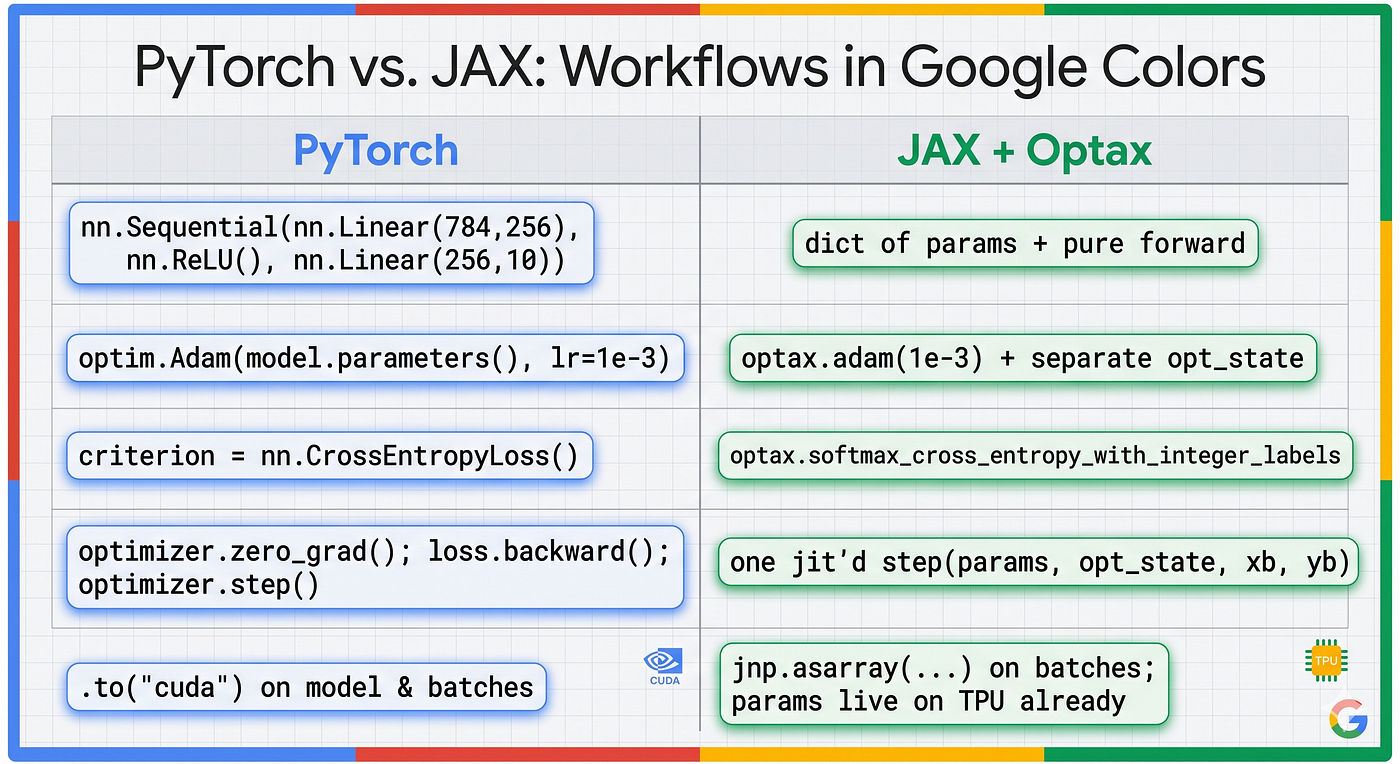
PyTorch → JAX cheat sheet (training-loop edition)

Things that go wrong

**ImportError: optax** — you forgot python3 -m pip install -U optax.

MNIST download times out. The Keras mirror is usually snappy, but if it’s slow, pre-download on your laptop and gcloud compute tpus tpu-vm scp it to the TPU.

First epoch slow, then hangs on epoch 2. You’re probably reconstructing the @jit inside the epoch loop — check that step is defined outside of it.

**opt_state not updating between epochs.** You ignored the return value from optimizer.update. Thread it through exactly like you thread params.

Loss goes to NaN immediately. Probably a data normalization issue — check that pixels are in [0, 1], not still in [0, 255].

The loop is much slower than 0.3s/epoch. Most likely you’re calling float(loss) or printing loss inside the inner loop, which forces a host sync every step. Accumulate the JAX arrays and sync once per epoch instead.

One model trained on one chip. In Part 6, we’ll delete this TPU, spin up a 4-chip v6e-4, and see how the same training code parallelizes — plus the dirty truth about when naive tensor parallelism actually slows you down. Then we’ll shut everything down and audit the bill.