Tabular Foundation Models, Part 2: Inside the Architecture

(Post #2 in the Tabular Foundation Models series)

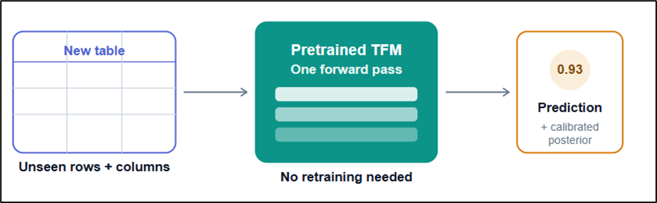
Part 1 of this series introduced the core ideas behind Tabular Foundation Models and explored how TabPFN brought the foundation-model paradigm to tabular data. We saw how a pretrained transformer could achieve competitive performance against tuned gradient-boosted trees without dataset-specific training or hyperparameter tuning. But an important question remained unanswered: Can this approach scale beyond small tabular datasets?

The original TabPFN was designed primarily for datasets with up to roughly 10,000 rows and 500 features. While that was enough to demonstrate the promise of in-context learning for tables, many real-world machine learning problems operate at a much larger scale.

In this post, we’ll go one level deeper and examine the architectural innovations that made the next generation of Tabular Foundation Models possible. We’ll explore why scaling TabPFN is challenging, how TabICL rethinks attention to handle larger datasets more efficiently, and how TabDPT takes a fundamentally different approach by learning from real-world tabular data rather than relying solely on synthetic datasets.

By the end, you’ll understand the key ideas behind these architectures, the trade-offs they make, and how the field evolved from proving that tabular foundation models can work to figuring out how far they can scale.

The Scaling Challenge Behind TabPFN

In Part 1, we saw how TabPFN demonstrated that in-context learning could be remarkably effective for tabular data. However, there was one important limitation we only briefly touched upon: scalability.

The original TabPFN and its successors were designed to be invariant to both row ordering and column ordering. This is a desirable property because, unlike text, tabular datasets have no natural sequence — there is no inherent reason why one row or feature should come before another. Achieving this invariance, however, comes at a cost.

TabPFN v2 represents tables at the cell level, treating each cell as a token rather than representing entire rows or columns. To capture relationships within the data, the model alternates between attending across features within a row and attending across rows within a feature. This design allows the model to effectively learn interactions across both dimensions of a table while maintaining permutation invariance. For small and medium-sized datasets, this approach works exceptionally well. The challenge emerges as the dataset size grows.

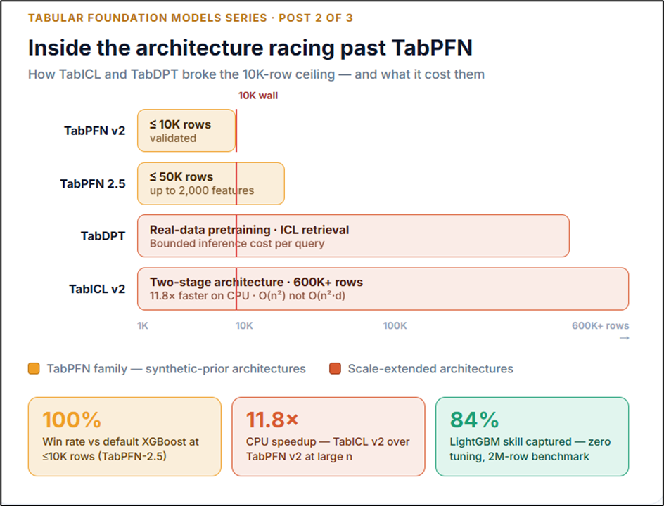
Because computation scales with the number of cells rather than simply the number of rows, the total number of tokens can increase dramatically. A dataset with 100,000 rows and 200 features contains 20 million cells, creating a computational burden that quickly becomes impractical for transformer-based architectures. As a result, while TabPFN v2 delivers strong performance on smaller datasets, scaling to larger tabular problems introduces significant memory and computational challenges.

How TabPFN v2’s Dual Attention Works

To understand why scaling becomes difficult, it’s worth taking a closer look at how TabPFN v2 processes tabular data. Unlike traditional tabular models that operate on rows, TabPFN v2 represents a dataset as a three-dimensional structure consisting of samples × features × embeddings. Both training examples and test examples are combined into a single context, allowing the model to perform in-context learning directly during inference. The key innovation is its dual-attention mechanism, which alternates between two complementary views of the data:

Row-Wise Attention

In the first step, attention is applied within each row.Here, every feature can interact with every other feature belonging to the same sample. This allows the model to learn relationships such as feature interactions, nonlinear dependencies, and cross-feature patterns that are specific to an individual observation. You can think of this as the model asking, “Given all the information available for this customer, patient, or transaction, how do these features relate to one another?”

Column-Wise Attention

In the next step, attention is applied within each column.Now, each value for a given feature can interact with the same feature across all other samples. This enables the model to understand how a feature behaves across the dataset and identify broader population-level patterns. At this stage, the model is effectively asking:“How does this feature vary across different examples, and what can that tell me about the current prediction task?”

Alternating Between Both Views

These two attention operations are stacked repeatedly across multiple layers. The model alternates between:

1. Understanding relationships within a sample (row-wise attention)
2. Understanding relationships across samples (column-wise attention)

Over successive layers, information propagates through both dimensions of the table, allowing the model to build a rich representation of the dataset without relying on any fixed row or column ordering. This design is what gives TabPFN v2 its desirable permutation invariance. Since rows and columns are treated as sets rather than sequences, predictions remain unchanged if the dataset is reordered.

Why This Becomes Expensive

The challenge is that attention is performed at the cell level rather than the row level. Instead of representing a table with 100,000 rows and 200 features as 100,000 tokens, the model effectively reasons over 20 million cells. As datasets grow, memory consumption and computational requirements increase rapidly, eventually becoming the primary bottleneck for scaling.

This creates the central tension in TabPFN v2: The same architectural design that provides permutation invariance and strong predictive performance on small datasets is also what limits scalability on larger ones.

Enter TabPFN-2.5

The latest generation, TabPFN-2.5, retains the same dual-attention foundation but introduces several improvements aimed at extending its practical limits. One particularly interesting addition is a set of learned “thinking rows” that are appended to the input during inference. Similar in spirit to the additional reasoning tokens used by modern LLMs, these learned rows provide extra computational workspace for the model without altering the underlying dataset.

Combined with other architectural improvements, TabPFN-2.5 significantly expands the range of datasets the model can handle, supporting up to roughly 50,000 samples and 2,000 features — a substantial increase over earlier versions.

However, even with these advances, the fundamental scaling challenge remains. The question researchers began asking was no longer whether in-context learning works for tabular data, but rather: Can we preserve its strengths while reducing the computational burden of dual attention?

Why Does the Cost Grow So Quickly?

The scaling limitations of TabPFN v2 become easier to understand when we look at the computational complexity of its dual-attention mechanism.The overall attention cost can be approximated as: O(n²d + nd²). The two terms correspond directly to the two attention operations we discussed earlier.

The Cost of Column-Wise Attention

Recall that during column-wise attention, each value in a feature column can attend to every other value in the same column. For a single feature, this requires comparing every row against every other row, resulting in a complexity of O(n²). Since this operation is performed across all d features, the total cost becomes: O(n²d). This is the term that typically dominates in practice.

The Cost of Row-Wise Attention

During row-wise attention, each feature interacts with every other feature within the same sample. For a single row, this requires: O(d²) operations. Since the computation is repeated across all n rows, the total cost becomes: O(d²n).

Why Rows Become the Bottleneck

The implications are straightforward:

• Double the number of rows → roughly 4× the column-attention cost
• Double the number of features → roughly 4× the row-attention cost

While both terms grow quadratically, real-world datasets often contain far more rows than features. A customer analytics dataset might contain hundreds of features but millions of rows. As a result, the (n² d) term tends to become the dominant bottleneck long before feature dimensionality becomes a problem. This explains why TabPFN performs exceptionally well on small and medium-sized datasets but becomes increasingly expensive as dataset size grows.

An Intuitive Example

Imagine increasing a dataset from 5,000 rows → 10,000 rows while keeping the number of features fixed. Although the dataset size only doubled, the cost of column-wise attention increases by approximately 4× because every row now needs to compare itself against four times as many row pairs.This is fundamentally different from tree-based methods such as XGBoost, whose computational costs grow much more gracefully with dataset size.

The Motivation for TabICL

This quadratic row-scaling behavior became one of the biggest obstacles preventing Tabular Foundation Models from being applied to larger real-world datasets.

In fact, the authors of TabICL observed that the performance advantage of their architecture over TabPFN grows as datasets become larger. For smaller datasets, the speedup is relatively modest, but as the number of rows increases and the quadratic attention term begins to dominate, the efficiency gains become much more significant.

This observation motivated a key question: Can we preserve the benefits of in-context learning while avoiding the quadratic dependency on the number of rows? TabICL’s architecture was designed specifically to answer that question.

TabICL’s Solution: Decoupling Rows from Features

If TabPFN’s scaling challenge comes from performing attention directly over individual cells, TabICL’s solution is surprisingly elegant:Compress first, perform in-context learning later. Rather than repeatedly applying row-wise and column-wise attention across an ever-growing grid of cells, TabICL separates the process into two distinct stages.

Stage 1: Build Row Representations The first stage focuses on understanding the structure of each row. Using a dedicated encoder, TabICL processes feature interactions within a row while also incorporating information about how those features behave across the dataset. The result is a fixed-dimensional embedding that summarizes the row. Think of this as converting a spreadsheet row with hundreds of features into a compact representation that captures its most important information.Once this step is complete, the original cell-level table is no longer needed.

Stage 2: Perform In-Context Learning on Row Embeddings The second stage is where in-context learning happens. Instead of operating on millions of individual cells, the transformer now works on a sequence of row embeddings, with each row represented by a single token. This dramatically reduces the computational burden. The model is no longer reasoning over a large grid of cells but over a much smaller set of row-level representations.

Why This Scales Better The key advantage is that the expensive row-attention computation is no longer tied to the number of features.For TabPFN, attention complexity scales approximately as: O(n²d + d²n) where: (n) = number of rows and (d) = number of features

For TabICL, the complexity becomes roughly: O(n² + nd²). The crucial difference is the disappearance of the feature dimension from the quadratic row-attention term. In practical terms, once rows have been compressed into embeddings, increasing the number of features no longer makes row-to-row attention more expensive. This significantly improves scalability for larger datasets.

What Does This Enable?

This architectural redesign allows TabICL to operate at scales that would be challenging for earlier TabPFN variants. The original TabICL was pretrained on synthetic datasets containing up to 60,000 samples and demonstrated the ability to handle datasets with hundreds of thousands of rows on commodity hardware. More recently, TabICLv2 extended this idea further through improved feature-grouping strategies that increase representation diversity without substantially increasing model size.

The result is a model that maintains the benefits of in-context learning while achieving substantially faster inference and training times on large datasets.

The Bigger Picture

TabPFN and TabICL ultimately share the same goal: learning a reusable inference procedure for tabular data through pretraining.

The difference lies in how they represent the table.

• TabPFN: performs attention directly on cell-level representations, maximizing expressiveness but limiting scalability.
• TabICL: compresses rows into embeddings first and then performs in-context learning, trading some architectural complexity for dramatically improved scalability.

This marks the first major branch in the evolution of Tabular Foundation Models: moving from proving that in-context learning works for tables to engineering architectures that can make it practical at scale.

TabDPT: Learning from Real Data Instead of Synthetic Worlds

While TabPFN and TabICL primarily focus on solving the scalability challenge, they still share a fundamental assumption inherited from the original PFN framework: Pretrain on synthetic datasets and transfer that knowledge to real-world problems. TabDPT takes a different path.

Rather than relying exclusively on synthetic datasets generated from structural causal models, TabDPT is pretrained on large collections of real-world tabular datasets gathered from sources such as OpenML. The motivation is simple: while synthetic data provides a clean and controlled training signal, it may not fully capture the complexity, noise patterns, and irregularities present in real-world data. The central hypothesis behind TabDPT is that exposure to diverse real datasets can teach useful patterns that are difficult to reproduce through synthetic generation alone.

Self-Supervised Learning for Tables

To make large-scale pretraining on real data possible, TabDPT adopts a self-supervised learning strategy inspired by advances in natural language processing. Instead of requiring labels, the model learns by reconstructing missing information within a table.

During training, selected column values are masked and hidden from the model. The model must then predict the missing values using the remaining features in the row along with contextual information from other rows in the dataset. If this sounds familiar, it’s because the idea closely resembles the masked-token prediction objective used by models such as BERT. Just as language models learn by filling in missing words, TabDPT learns by filling in missing cells.

Retrieval Instead of Full-Dataset Context

TabDPT introduces a second key innovation: retrieval-based in-context learning. One of the challenges with foundation models for tabular data is that providing an entire training dataset as context quickly becomes infeasible as datasets grow larger.

TabDPT addresses this by retrieving a small set of relevant examples for each query row rather than processing the full dataset. The model then performs in-context learning using only this retrieved subset. The intuition is similar to retrieval-augmented generation (RAG) systems used in modern LLM applications: instead of consulting everything, retrieve the most relevant information and reason over that.

This design keeps computational costs bounded even when the underlying dataset contains millions of rows.

A Different Scaling Strategy

What makes TabDPT particularly interesting is that it shifts the conversation from architectural efficiency to data scaling. Rather than asking:“How can we make attention more efficient?” TabDPT asks:“What happens if we train larger models on more real-world tabular data?”

The authors report a clear scaling trend: increasing model size and pretraining data consistently improve downstream performance, following predictable scaling behaviors similar to those observed in modern language models.

If these trends continue to hold, they suggest a potentially important direction for the future of Tabular Foundation Models: not just better architectures, but larger models trained on increasingly diverse collections of real-world tabular data.

Two Paths Toward Scale

At this point, the field has begun to diverge into two complementary strategies:

• TabICL: Improve scalability through architectural innovation, compressing tables into row-level representations before performing in-context learning.
• TabDPT: Improve scalability through large-scale self-supervised pretraining on real-world tabular datasets combined with retrieval-based context selection.

Both approaches aim to push beyond the limitations of the original TabPFN, but they represent fundamentally different bets on where the future of tabular foundation models lies.

Enterprise Reality Check: What Happens at Million-Row Scale?

Much of the research around Tabular Foundation Models focuses on benchmark datasets, but the real test comes when these models are applied to production-scale business problems. One of the most interesting case studies comes from a credit risk team at Mission Lane, which evaluated TabICL on a large proprietary credit dataset containing over 2 million training records, nearly 1 million holdout records, and approximately 300 features.

This setup immediately exposed one of the practical challenges of in-context learning at scale. While TabICL is designed to handle much larger datasets than TabPFN, providing millions of records as context is still computationally infeasible. Instead, the team experimented with different context window sizes ranging from hundreds to hundreds of thousands of examples to identify an effective operating point. Their findings revealed an important trade-off.

On the accuracy front, the results were encouraging. Using a context window of around 60,000 examples, TabICL achieved performance that approached that of a highly optimized production LightGBM model trained on the full dataset. Remarkably, this was achieved without extensive hyperparameter tuning, highlighting one of the key promises of foundation models for tabular data. However, predictive performance was only half the story.

When the team evaluated inference latency, traditional gradient-boosted trees retained a significant advantage. LightGBM remained dramatically faster than TabICL, particularly in real-time prediction scenarios where individual predictions must be served with extremely low latency. While TabICL demonstrated competitive predictive power, the computational overhead of in-context learning made deployment considerably more expensive.

The Key Lesson

This case study highlights a recurring theme in the current generation of Tabular Foundation Models:

Accuracy is becoming increasingly competitive. Serving efficiency is not.

For many enterprise applications, model quality is only one part of the equation. Latency requirements, infrastructure costs, throughput constraints, and operational complexity often matter just as much as predictive performance. As a result, the most promising near-term use cases for TFMs may not be direct replacements for production gradient-boosted trees. Instead, they may serve as powerful foundation models that can later be fine-tuned, distilled, or compressed into more efficient deployment architectures.

This tension between model quality and serving cost is likely to shape the next phase of innovation in tabular foundation models — and it provides a natural bridge to the next part of this series, where we’ll explore fine-tuning, distillation, and deployment strategies designed to bring TFM-level performance closer to production-friendly latency.

Common Pitfalls and Failure Modes

As Tabular Foundation Models continue to mature, many of the mistakes practitioners make are no longer about model accuracy — they’re about understanding the trade-offs that come with scaling and deployment.

1. Confusing Scalability with Efficiency

A model that can handle hundreds of thousands of rows is not necessarily a model that can process them efficiently. Architectures such as TabICL were explicitly designed to support much larger datasets than TabPFN. However, operating at the upper end of their supported range may introduce increased computational costs and, in some cases, diminishing accuracy gains. Always validate performance at your target dataset size rather than assuming the architecture’s maximum supported scale is also its optimal operating point.

2. Treating Caching as a Free Optimization

Many TFM implementations support techniques such as KV (Key-Value) caching to accelerate repeated inference. While caching can significantly reduce latency for repeated predictions against a fixed reference dataset, it introduces additional memory overhead and operational complexity. The benefits are often workload-dependent, particularly when the underlying reference data changes frequently. Measure the trade-off before incorporating caching into a production design.

3. Optimizing for Accuracy While Ignoring Latency

One of the most common evaluation mistakes is focusing exclusively on benchmark metrics such as ROC-AUC while overlooking inference speed. For many enterprise applications — credit scoring, fraud detection, recommendation systems, and risk models — serving latency can be just as important as predictive performance. A model that achieves marginally higher accuracy may still be impractical if it significantly increases infrastructure costs or response times.

Always benchmark both batch inference and single-record inference, as their performance characteristics can differ dramatically.

4. Assuming Real-Data Pretraining Solves Distribution Shift

TabDPT’s use of real-world datasets represents an important step forward, but it does not eliminate distribution shift. The model’s prior knowledge is still shaped by the datasets it encountered during pretraining. If your domain differs substantially from those distributions, performance may be less reliable than expected. Retrieval-based approaches help, but they remain dependent on the relevance of the retrieved examples.

5. Relying on Outdated Benchmarks

The TFM ecosystem is evolving rapidly. New model variants, architectural improvements, and benchmark results appear every few months. Performance comparisons that were accurate six months ago may already be outdated. Whenever possible, rely on recent evaluations and validate claims on your own datasets rather than assuming historical rankings still hold.

Best Practices Checklist

The broader lesson is that scaling tabular foundation models is no longer purely a research problem — it is increasingly an engineering problem. As architectures improve, the key questions are shifting from “Can these models work?” to “Can they deliver their benefits efficiently in real-world production systems?”

Where This Leaves Us

One of the most interesting takeaways from the evolution of Tabular Foundation Models is that there isn’t a single path to scaling in-context learning for tabular data. Each architecture we’ve explored in this post tackles the challenge from a different angle:

• TabPFN v2 prioritizes rich representations and permutation invariance, delivering strong performance on small to medium-sized datasets.
• TabICL focuses on scalability, redesigning the architecture to handle significantly larger datasets by compressing rows before performing in-context learning.
• TabDPT takes a different route altogether, leveraging real-world data and self-supervised learning to move beyond the limitations of purely synthetic pretraining.

At the same time, the Mission Lane case study highlighted an important reality: while the accuracy of modern TFMs is becoming increasingly competitive with traditional approaches, serving latency remains a major challenge — particularly for real-time production systems. That challenge sets the stage for the next chapter in the story.

In Part 3, we’ll explore how practitioners are addressing the deployment gap through techniques such as fine-tuning, distillation, and embedding extraction. The goal is simple: retain the strengths of Tabular Foundation Models while achieving the efficiency required for real-world production environments. In other words, if Part 1 was about proving that Tabular Foundation Models can work, and Part 2 was about making them scale, Part 3 is about making them deployable.