Exploring Flight Delay Data

Part 3 in Predicting Flight Delays

With my newly scraped data in hand, I can now move on to data exploration to make sure I understand what I have to work with before cranking it through cleaning and model training. All code can be found on my github https://github.com/dlosowyj/flight-delay-forecasting.

Data Summary

First thing’s first, what kind of data do we have? While it would be nice to take a look at all 33 airports at once, my computer is not up to that task and it would hamper my exploration of the data by starting too big too soon. Instead, I will be starting with just PDX.

(At this point I should also note that I will not be splitting my data into a training and test set for this exploration. My goal is simply to observe existing correlations among the data and not to do any feature engineering so I am not concerned about data leakage affecting my final model.)

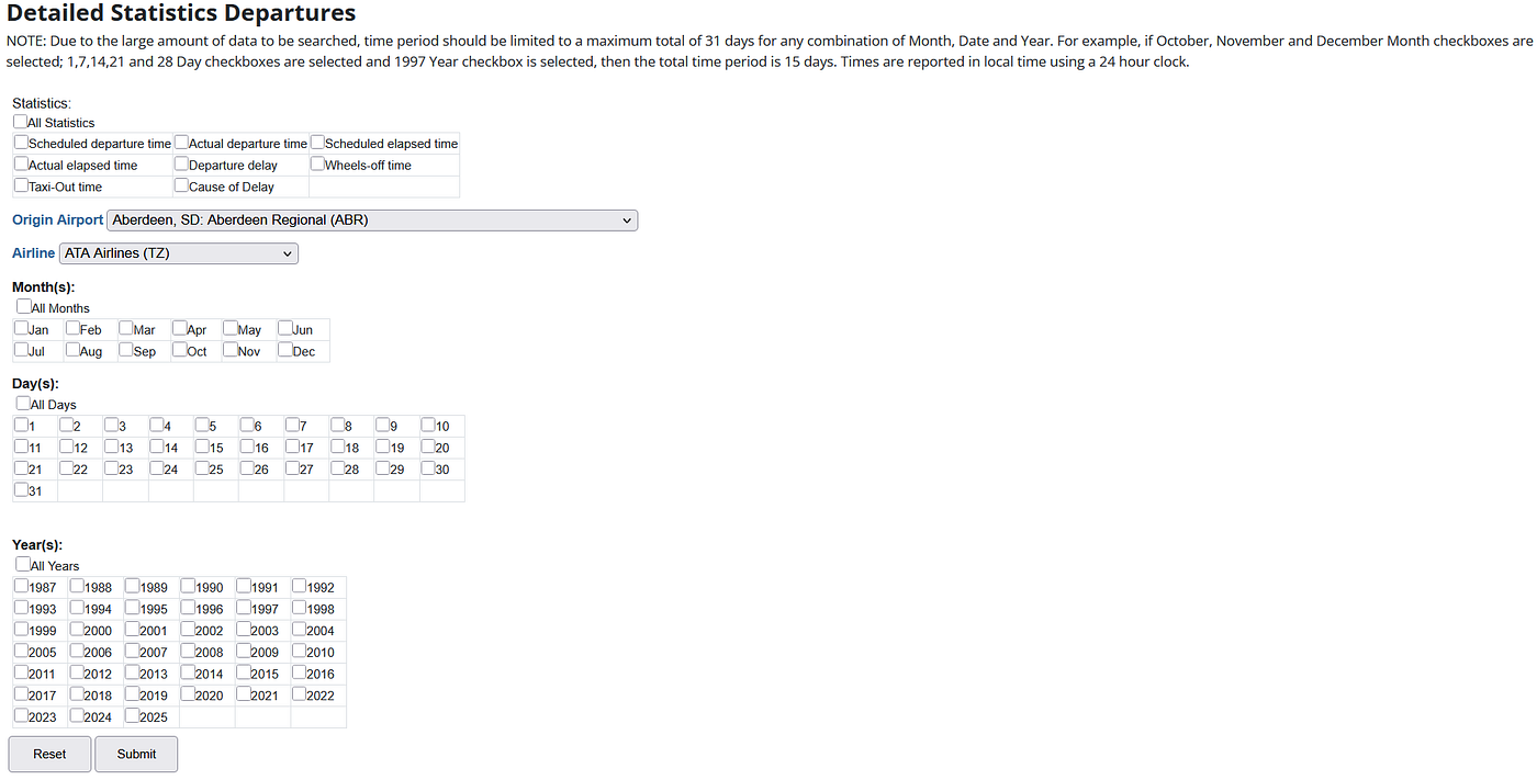
Part 2’s web scraping resulted in one file per airport-airline combination. Behind the scenes, I have since concatenated the data for PDX so that delays for all carriers are now housed in a single file. Loading that file into a DataFrame, I can take a look at what features we have to explore.

import pandas as pd

delay_df = pd.read_csv('C:/Users/dloso/Documents/Data Science/flight-delay-forecasting/data/delays/concatenated_delays/PDX_delays.csv')
delay_df.info()

<class 'pandas.core.frame.DataFrame'>
RangeIndex: 594126 entries, 0 to 594125
Data columns (total 18 columns):
 #   Column                                    Non-Null Count   Dtype  
---  ------                                    --------------   -----  
 0   Unnamed: 0                                594126 non-null  int64  
 1   Carrier Code                              594126 non-null  object 
 2   Date (MM/DD/YYYY)                         594126 non-null  object 
 3   Flight Number                             594126 non-null  float64
 4   Tail Number                               593220 non-null  object 
 5   Destination Airport                       594126 non-null  object 
 6   Scheduled departure time                  594126 non-null  object 
 7   Actual departure time                     594126 non-null  object 
 8   Scheduled elapsed time (Minutes)          594126 non-null  float64
 9   Actual elapsed time (Minutes)             594126 non-null  float64
 10  Departure delay (Minutes)                 594126 non-null  float64
 11  Wheels-off time                           594126 non-null  object 
 12  Taxi-Out time (Minutes)                   594126 non-null  float64
 13  Delay Carrier (Minutes)                   594126 non-null  float64
 14  Delay Weather (Minutes)                   594126 non-null  float64
 15  Delay National Aviation System (Minutes)  594126 non-null  float64
 16  Delay Security (Minutes)                  594126 non-null  float64
 17  Delay Late Aircraft Arrival (Minutes)     594126 non-null  float64
dtypes: float64(10), int64(1), object(7)
memory usage: 81.6+ MB

Examining Possible Model Features

The features that first jump out at me are the Carrier Code, Date (MM/DD/YYYY), Scheduled departure time, and Departure delay (Minutes). There are other features that include “delay” in the title, but these are all subsets of the overall delay. For instance, Delay Carrier (Minutes) is a measure of the delay attributable to carrier-controlled elements like availability of a flight crew to man a plane on time. Incorporating this feature (or other delay features) would be similar to including Departure delay (minutes) itself in our model. At that point the model no longer needs to predict a delay since I would have given it the answer directly.

Before going further, I am just going to do a quick describe() check on the Date (MM/DD/YYYY), Scheduled departure time, and Departure delay (Minutes) to see what I am working with. The date range is as expected — it covers January 1, 2021 to September 30, 2025 and the departure times similarly cover the whole day, which makes sense. The delay times, however, do have an incredibly large maximum value of nearly 2 days, a value that does not seem reasonable. I will make sure to drop values larger than 24 hours when cleaning the data later.

delay_df['Date (MM/DD/YYYY)'] = pd.to_datetime(delay_df['Date (MM/DD/YYYY)'])
delay_df['Scheduled departure time'] = pd.to_datetime(delay_df['Scheduled departure time'], format='%H:%M')
delay_df[['Date (MM/DD/YYYY)', 'Departure delay (Minutes)', 'Scheduled departure time']].describe()

       Date (MM/DD/YYYY)   Departure delay (Minutes)  Scheduled departure time
count  594126              594126.000000              594126
mean   2023-07-07 13:59:46 10.814613                  1900-01-01 13:23:25
min    2021-01-01 00:00:00 -60.000000                 1900-01-01 00:04:00
25%    2022-05-20 00:00:00 -4.000000                  1900-01-01 09:00:00
50%    2023-07-29 00:00:00 0.000000                   1900-01-01 13:10:00
75%    2024-09-02 00:00:00 11.000000                  1900-01-01 17:35:00
max    2025-09-30 00:00:00 3024.000000                1900-01-01 23:59:00
std    NaN                 39.733229                  NaN

Looking at the features that we have initially identified as important, if we plot whether a flight is delayed (0 is on-time, 1 is delayed) against carrier, day of departure, and hour of departure, we can already see some strong trends developing. Several carriers have more on-time flights than delayed ones, however, Southwest Airlines (WN) clearly bucks that trend thereby making it an important predictor.

Similarly for the day of departure, there appears to be a strong uptick in delays in the summertime, possibly due to the larger total number of flights during that period. A higher volume of aviation traffic would mean smaller margins of errors on flights before delays start to increase. For example, a small delay in a ground crew during the slower winter months could be absorbed by an airport since there would be other gates open, but the same delay in the busier summer would cause cascading delays.

Then the relationship between delays and hour of departure shows a marked increase in the number of delays later in the day as compared to the morning. This is likely influenced by flight crews getting delayed throughout the day and those effects compounding for later flights.

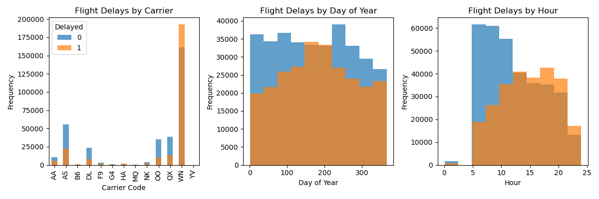
Flight delays by carrier, day of departure, and hour of departure.

All three of these features appear quite useful for our model, but what about other fields like the Destination Airport? Is it possible that flights are delayed more often when traveling to specific destinations? I can investigate this by calculating the proportion of flights that are delayed depending on the destination with panda’s groupby() and value_count() functions. Sorting by the proportion of delayed flights, I see that there is a strong correlation between the destination airport and flight delays so this feature should certainly be included in my initial model testing. (As an aside, PDX shows up in the Destination Airport feature, which is unexpected. I will keep this in mind during data cleaning.)

delay_df['Delayed'] = np.where(delay_df['Departure delay (Minutes)'] > 0, 1, 0)

dest_act_df = pd.DataFrame(delay_df.groupby('Destination Airport')['Delayed'].value_counts())
dest_prop_df = pd.DataFrame(delay_df.groupby('Destination Airport')['Delayed'].value_counts(normalize=True))
dest_df = pd.concat([dest_act_df, dest_prop_df], axis=1)
dest_df.columns = ['Count', 'Proportion']
dest_df = dest_df.reset_index()
dest_df = dest_df[dest_df['Delayed'] == 1]
print(dest_df.sort_values(by='Proportion', ascending=False).head(20))

      Destination Airport  Delayed  Count  Proportion
34                  CLE        1      1    1.000000
155                 PBI        1      4    0.800000
157                 PDX        1    365    0.762004
121                 MEM        1   1327    0.647001
105                 LGA        1   3874    0.642029
24                  BUF        1     17    0.629630
127                 MKE        1   1034    0.629337
175                 RDU        1    992    0.625473
179                 RSW        1    570    0.615551
37                  CMH        1   1087    0.613085
45                  DAL        1    339    0.603203
93                  JAX        1    336    0.600000
107                 LGB        1   1433    0.599833
28                  BWI        1   4762    0.594433
119                 MDW        1   7746    0.594018
213                 TPA        1   3499    0.584238
91                  IND        1   1589    0.579082
32                  CHS        1    928    0.573902
159                 PHL        1    318    0.569892
111                 LIT        1   2515    0.564534

The Tail Number could also prove crucial in determining the likelihood of a flight delay. Imagine, say, an older aircraft that needs more consistent maintenance leading to repeat delays between flights. Using my procedure from above, I do indeed find that some planes are much more likely to be delayed than others making it another good feature candidate for the model.

tail_no_act_df = pd.DataFrame(delay_df.groupby('Tail Number')['Delayed'].value_counts())
tail_no_prop_df = pd.DataFrame(delay_df.groupby('Tail Number')['Delayed'].value_counts(normalize=True))
tail_no_df = pd.concat([tail_no_act_df, tail_no_prop_df], axis=1)
tail_no_df.columns = ['Count', 'Proportion']
tail_no_df = tail_no_df.reset_index()
tail_no_df = tail_no_df[tail_no_df['Delayed'] == 1].sort_values(by='Proportion', ascending=False)
print(tail_no_df[tail_no_df['Count'] > 20].head(20))

       Tail Number  Delayed  Count  Proportion
2475      N391HA        1     43    0.704918
4752      N745SW        1    113    0.693252
2405      N382HA        1     38    0.678571
6756      N8941Q        1     35    0.673077
4502      N711HK        1     84    0.666667
2451      N388HA        1     41    0.661290
2429      N385HA        1     37    0.660714
4567      N717SA        1     98    0.657718
2437      N386HA        1     44    0.656716
6766      N8946L        1     40    0.655738
2514      N396HA        1     34    0.653846
6434      N8808Q        1    313    0.653445
2389      N380HA        1     30    0.652174
6764      N8945Q        1     33    0.647059
6428      N8805L        1    309    0.646444
6426      N8804L        1    307    0.643606
6746      N8938Q        1     32    0.640000
6180      N8707P        1    220    0.639535
6784      N8953Q        1     23    0.638889
6792      N8957Q        1     23    0.638889

Caution About Collinearity

Finally, it is tempting to repeat this procedure for the flight number, but there are two risks to this:

1. The flight number for a trip between two cities at a given time is not necessarily the same across the years so I cannot depend on this to be identical across our dataset.
2. Even if the flight number was constant, that feature would be highly correlated with the destination airport and departure date/time. Since I am already including those other features, I do not need to introduce a highly collinear one to our analysis.

I can quickly check 2. using a chi-squared analysis of our data and it yields a p-value of 0.0 suggesting that Flight Number and Destination Airport are not independent. While this does not tell me the strength of the relationship, it does lend credence to my concerns about collinearity so I will not be including it in the model.

from scipy.stats import chi2_contingency

contingency_table = pd.crosstab(delay_df['Flight Number'], delay_df['Destination Airport'])

chi2_statistic, p_value, dof, expected_freq = chi2_contingency(contingency_table)

print(f'\nChi-squared Statistic: {chi2_statistic}')
print(f'P-value: {p_value}')

Chi-squared Statistic: 25075278.337462157
P-value: 0.0

Summary

Now that I have examined the dataset, there are some clear features to test out in the classification model. Specifically, I will be testing the following:

• Carrier Code
• Day of Departure
• Hour of Departure
• Destination Airport
• Tail Number.

I also noted that while an additional feature like Flight Number could prove useful, I will be avoiding its inclusion in the model testing to avoid collinearity with other existing features. There is no need to include extra data in the model that does not include new information. It will just slow down fitting!

Other Flight Delay Posts

Part 1: Predicting Flight Delays Intro.

Part 2: Web Scraping Flight Delay Data

Part 4: Data Cleaning for Classification of Flight Delays

Part 5: Testing ML Models for Classification of Flight Delays

Part 6: A Random Forest Model for Flight Delay Classification