Machine Learning Algorithms

How AdaBoost Works: Turning Weak Learners into Strong Predictors

Understanding the Step-by-Step Process and Inner Workings Behind AdaBoost’s Predictive Power in Binary Classification

Introduction

AdaBoost (short for Adaptive Boosting) is a machine learning classification model that falls under the category of boosting algorithms, formulated by Yoav Freund and Robert Schapire in 1995. AdaBoost works by combining multiple weak classifiers to create a strong classifier by iteratively adjusting the weights of training samples. Usually the weak classifiers used in AdaBoost are decision stumps — simple decision tree classifiers with a maximum depth of 1. Despite their simplicity, when combined through AdaBoost, these weak classifiers can produce highly accurate models for complex tasks.

In the case of binary classification, AdaBoost uses the classes -1 and +1, where -1 represents the negative class (often mapped to 0 in real-world applications) and +1 represents the positive class (often mapped to 1). Popular machine learning libraries, such as scikit-learn, automatically handle the mapping from -1 and +1 to the actual class labels in the data.

AdaBoost trains classifiers in a stage-wise, additive manner. Initially, a classifier is trained on the data, and weights are calculated for each sample. The weighted data is then used to generate a new subset of data, which is fed into the next classifier. This process is repeated iteratively until the final classifier is trained. The results from all classifiers are then combined to produce the final prediction.

How AdaBoost Works?

Geometric Perspective:

Consider an AdaBoost algorithm with three decision tree classifiers (the number can vary), each with a maximum depth of 1. Suppose we train this classifier on some data, which generates a boundary line vertically along the y-axis, separating the positive and negative classes. According to this classifier, points in the green-colored region are classified as belonging to the positive class, while points in the red-colored region are classified as belonging to the negative class, as shown in Figure 1 below.

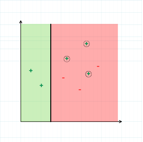
Fig. 1: Decision Tree Classifier 1 — Classification Boundary and Class Regions

From the figure above, we can clearly see that the three encircled points, which belong to the positive class, are incorrectly classified as negative by the first decision tree classifier. As a result, higher weights will be assigned to these misclassified points to force the model to classify them correctly. A new subset of the data will then be derived based on these updated weights (the process of weight calculation and how the subset of data is derived will be discussed in a later section). This derived data will then be passed on to the next classifier.

The updated data is then passed to the second decision tree classifier, where, again, the boundary line is drawn vertically, parallel to to the y-axis, separating the positive and negative classes, as shown in Figure 2 below.

Fig. 2: Decision Tree Classifier 2 — Classification Boundary and Class Regions

From the figure above, we can clearly see that the two encircled points, which belong to the negative class, are now incorrectly classified as positive by the second decision tree classifier. These points will now be assigned higher weights to force the model to classify them correctly. The process of deriving a new subset of the data based on these updated weights will then be repeated.

The derived data is then given to the third and final decision tree classifier, where, this time, the boundary line is drawn horizontally, parallel to the x-axis, separating the positive and negative classes, as shown in Figure 3 below.

Fig. 3: Decision Tree Classifier 3 — Classification Boundary and Class Regions

This time, we can see that the three encircled points, which belong to the positive class, are incorrectly classified as negative by the third decision tree classifier.

At this point, a question arises: why have we trained multiple decision trees if none of them is performing better individually? This is where AdaBoost comes into play. AdaBoost combines these three models and defines a more optimal boundary, resulting in significantly improved performance, as shown in Figure 4 below.

Fig. 4: AdaBoost— Classification Boundary and Class Regions

To summarize, AdaBoost works by combining multiple weak classifiers to create a strong classifier by iteratively adjusting the weights of training samples.

Mathematical Perspective:

To better understand the AdaBoost algorithm, let us consider a simple dummy dataset. This dataset consists of two input columns (X1 and X2) and one output column (y), with a total of 5 rows, as illustrated in Figure 5 below.

Fig. 5: Original Dataset

Initially, the same weight will be assigned to each row, which can be calculated as:

Weight = 1 / Number of rows

Fig. 6: Original Dataset with Weights Column

The weights column will not be used during training but is included in the figure solely to help understand how the algorithm works. The input features (X1 and X2) and the output feature (y) will now be passed to Decision Tree Classifier 1 to predict the output, as illustrated in Figure 7 below.

Fig. 7: Original Dataset with Weights Column and Prediction Column

You can clearly observe that Row 2 and Row 3 have been misclassified by the model. Based on these misclassified rows, we will calculate new weights. However, before calculating the weights, let us first understand some important concepts that will help us comprehend the process of weight calculation.

Error Rate (ε)

To calculate the weights, we first need to compute alpha (α). Alpha (α) requires the error rate (ε), which is calculated as:

Error Rate (ε) = Number of Misclassified Rows / Total Number of Rows

In this case, there are two misclassified rows out of a total of five rows. Hence, the error rate (ε) is: Error Rate (ε) = 2 / 5 = 0.4

Alpha (α)

Once the error rate (ε) is calculated, we can compute alpha (α) using the formula:

Alpha (α) = 1/2 ln [ ( 1- error rate (ε) ) / error rate (ε) ]*

Weights Calculation

When calculating and updating weights, it is important to note that we update the weights for both misclassified and correctly classified rows. The weights of the misclassified rows will be increased, while the weights of the correctly classified rows will be decreased.

For correctly classified rows, the formula to calculate the new weight is:

New Weight = Current Weight e^α*

For misclassified rows, the formula to calculate the new weight is:

New Weight = Current Weight e^-α*

After calculating the new weights using the formulas above, we observe that the sum of these weights is not equal to 1. Therefore, we need to normalize the weights by dividing each new weight by the sum of the newly calculated weights, as shown in Figure 8 below.

Fig. 8: Original Dataset with Weights, Prediction, New Weights and Normalized Weights Columns

Now, we need to convert the normalized weights column into a range. The range will be calculated as follows:

First Row:

• The range starts at 0.
• The end of the range is equal to the value of the first row’s Normalized Weight.

Second Row:

• The range starts from the upper bound of the previous row’s Range column.
• The end of the range is the value of the current row’s Normalized Weight added to the upper bound of the previous row’s Range column.

Subsequent Rows:

• The range starts from the upper bound of the previous row’s Range column.
• The end of the range is the value of the current row’s Normalized Weight added to the upper bound of the previous row’s Range column.

Last Row:

• The range starts from the upper bound of the previous row’s Range column.
• The end of the range is 1.

The process is shown below in Fig 9 below.

Fig. 9: Dataset with Range Column

Now that the Range column is derived, we need to generate 5 random numbers between 0 and 1, as we have 5 rows in the dataset. Let the random numbers be: [ 0.13, 0.43, 0.62, 0.50, 0.8 ] (corresponding to specific rows).

For each random number, check which range it falls into and identify the corresponding row.

• 0.13 belongs to Row 1.
• 0.43 belongs to Row 3.
• 0.62 belongs to Row 3.
• 0.50 belongs to Row 3.
• 0.8 belongs to Row 4.

Based on the above information, we will now create a subset of the dataset, which will consist of 5 rows: Row 1, Row 3, Row 3, Row 3, and Row 4, as shown in Figure 10 below.

Fig. 10 New Dataset

This marks the first iteration. The process will be repeated for all classifiers: training each classifier on the updated data, making predictions, calculating error rates, computing alpha, updating the weights, normalizing the weights, calculating the ranges, and deriving the new data. This cycle continues until the final classifier is trained.

How AdaBoost Combines Classifiers: The Final Prediction Process

Once all classifiers are trained, we combine them using the following formula:

p = α1 h1( x ) + α2 h2( x ) + α3 h3( x )*

• α₁: Alpha value for the first dataset (Classifier 1).
• h₁(x): Output prediction of the first classifier.
• α₂: Alpha value for the second dataset (Classifier 2).
• h₂(x): Output prediction of the second classifier.
• α₃: Alpha value for the third dataset (Classifier 3).
• h₃(x): Output prediction of the third classifier.

Finally, the final prediction is determined by the sign of p. If p is positive, the row is assigned to the positive class, as per the AdaBoost algorithm. If p is negative, the row is classified as belonging to the negative class.