Object Counting on Construction Sites with YOLO26 + SAHI

The story of a computer vision project from idea to live app: finding data, training on Colab, crashing kernels, a first test stuck at 72%, and the code that changed everything.

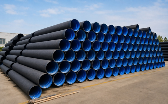
Pipe stack photo

🔗 Live app: https://yolo-construction-material-counter.streamlit.app

💻 Source code + training notebook: https://github.com/fhattat/YOLO-construction-material-counter

Introduction: A Question Left on the Job Site 26 Years Ago

Anyone who has worked on a construction site knows: counting materials is one of those invisible yet always-needed, critical tasks of the profession. Did the delivered material arrive complete? How much will be returned when the job wraps up? The questions are simple, the answers are hard — because in front of you sit hundreds of pieces stacked side by side, one on top of another. You count, lose track somewhere, go back to the start and count again. I lived this frustration first-hand in the early years of my career. In that moment, the same thought always crosses your mind: “I wish I could get this counted automatically.” I am actually a civil engineer. I graduated 26 years ago; for the last 18 years, I have been working in deep learning. This project was born right where those two worlds intersect.

What was once a wish is now something technology can genuinely deliver. And the materials to count are not just one type: PVC corrugated pipes, cement bags, concrete culverts… Even though I have not been in the field for many years, solving such a concrete problem of my first profession with my current expertise gives me a special kind of joy. Object counting had to start somewhere — so I started with one of the most frequently counted materials on site: PVC pipes.

How Big Is the Problem, Really?

In the construction industry, material inventory is usually kept in Excel sheets. Counting hundreds of stacked PVC pipes by hand takes many minutes; if two people count, you will most likely get two different results. A counting error means a “did material go missing, or did less arrive?” argument on site — and that argument costs far more than the count itself.

Yet today, the same job can be done from a phone photo: shoot, upload, get the result. In this article, I will walk through how I built a system that does exactly that. The outcome: 97% counting accuracy on a dense stack of 132 pipes, and a live web application anyone can use.

And the approach is not limited to pipes. Concrete culverts, cement bags, brick pallets, rebar bundles… Any material that gets stacked and needs counting can be counted with the same architecture. In industry terms: counting drops from minutes to seconds, the error margin stops depending on who counts, and the inventory record is documented with a photo.

The Architecture Decision: Why Both YOLO and SAHI?

Why isn’t YOLO enough on its own?

The first solution that comes to mind looks simple: train an object detection model (YOLO), count the boxes it finds, done.

But dense scenes hide a problem. Before processing, YOLO downscales the image to a fixed size (960 pixels in our model). In a 4000-pixel site photo, a pipe end in the back row shrinks to 5–10 pixels after downscaling. At that size, no pattern or texture is left — the model can no longer recognize it as a pipe. The large pipes in front get counted; the ones in the back silently disappear. And you receive no error message; you just see a smaller number.

What does SAHI do?

SAHI (Slicing Aided Hyper Inference) is not a model but an inference strategy. It wraps around YOLO and does three things:

1. Splits the photo into overlapping 512×512 slices
2. Runs YOLO on each slice separately — that 8-pixel pipe in the back appears 50+ pixels in its own slice and is detected with ease
3. Maps all detections back to the original photo’s coordinates; since slices overlap, pipes detected twice at slice borders are reduced to one via NMS (non-maximum suppression)

SAHI flow diagram — slicing → detection per slice → merging

My favorite analogy: YOLO is the eye, SAHI is the magnifying glass that brings that eye close to every corner of the photo. Of course, there is a cost; dozens of slices mean dozens of separate model calls, which means slower inference. But in a job where counting accuracy is critical, this trade-off will work strongly in your favor.

Data: Roboflow Universe Instead of Labeling from Scratch

Before starting to label my own dataset, I searched for existing data and found the p15-pipe dataset on Roboflow Universe: 4,500+ labeled pipe images, augmented, CC BY 4.0 licensed. Weeks of labeling work was wrapped up by a half-hour search with the right keywords (“pipe counting”, “pipe stack”, “circle-pipe”). There were many other datasets on the platform, but based on my experience, I tried to pick the one that best matched the kinds of stacks you would actually encounter on a construction site. You can, of course, also build your own dataset with plenty of photos taken in the field.

A small but instructive detail: the dataset had a v10, but a ready-trained model on Roboflow existed only for v9. I tried using the hosted model via the API; first a “model not found” (404) error, then GPU dependency issues (pycuda) — at which point I decided that training my own model would be both cleaner and more instructive. That way, control stayed entirely with me.

Training: Colab, Crashing Kernels, and the Lifesaving resume=True

I trained the model on Google Colab (T4 GPU): YOLO26-nano, 4,215 training images. I should note upfront that I solved some of the obstacles below with GPU capacity purchased through Colab’s “pay as you go” option.

Obstacle 1: The silent kernel crash

The first training attempt crashed without even an error message — the kernel silently restarted. The reason: free Colab’s ~12 GB of system RAM could not handle the imgsz=1280 + batch=8 + 8 parallel dataloaders combination. The RAM-safe recipe:

model.train(
    data=DATA_YAML,
    epochs=100,
    imgsz=960,      # instead of 1280
    batch=4,        # instead of 8
    workers=2,      # instead of 8
    cache=False,
    max_det=1000,   # critical — explained below
    patience=25,
)

Obstacle 2: The sneaky max_det=300 default

By default, YOLO returns at most 300 detections per image. In a scene containing more than 300 pipes, even if the model works flawlessly, the count gets stuck at 300 — and there is no warning telling you this. Anyone building a counting project needs to raise max_det.

Obstacle 3: Session cut-off

Colab cut the training at epoch 33. Luckily, I had been writing outputs to Google Drive from the very beginning; two lines resumed right where it left off:

model = YOLO('/content/drive/MyDrive/runs_boru/faz1/weights/last.pt')
model.train(resume=True)

If you run long trainings on Colab, Drive backup is not a “nice to have” — it is mandatory. A session drop is not a mere possibility; it is the likely outcome.

Training finished at epoch 68 with early stopping. Validation results:

mAP@50: 0.948

mAP@50–95: 0.668

The story these two numbers tell: the high mAP@50 (94.8%) says the model is very good at finding pipes, which is what matters most for counting. The lower mAP@50–95 means the boxes do not fit millimeter-perfect; that would be a concern in a classification or measurement project, but when the question is “how many pipes are there?”, a box being 5 pixels too wide does not change the answer. In counting projects, the metric to actually track is not mAP but MAE (the gap between the predicted count and the true count) — we will see it in the field shortly.

Training curves

First Test: 95 of 132 Pipes — and the Real Lesson

When I first tested the trained model with SAHI, the result was disappointing: 95 of 132 pipes were found (72%). The misses were not from random spots — shaded pipes at the right edge and pipe ends seen at oblique angles.

Most people’s first reflex would be “more data, longer training.” I first tried improvements that require no training at all. Two discoveries changed everything.

Discovery 1: A systematic parameter sweep

I swept the confidence threshold × slice size × overlap combinations in a loop:

for conf in [0.15, 0.20, 0.25, 0.30]:
    for slice_px in [384, 512, 640]:
        for overlap in [0.2, 0.3]:
            # count with each combination, compare to ground truth

Lowering the confidence threshold and shrinking the slice size pushed the count up to 118. But something odd sat in the table: slice=512 and slice=640 produced identical results. Why?

Discovery 2: Image scale is everything

My test image was a 469×293-pixel preview image. A 640-pixel slice is larger than a 469-pixel image — meaning SAHI was not slicing at all. The entire slicing architecture had been silently disabled.

The fix turned out to be remarkably simple: increase the image resolution.

big = cv2.resize(img, None, fx=3, fy=3, interpolation=cv2.INTER_CUBIC)

3x upscaling adds no new information to the photo — but it fixes two things at once: pipe ends approach the scale the model saw during training, and SAHI gets room to slice. The results:

• First test (default settings): 95/132 — 72%
• After the parameter sweep: 118/132 — 89%
• 3x upscale + optimal settings: 128/132 — 97%

From 72% to 97% without any retraining. The clearest lesson this project taught me: sometimes the biggest gain hides not in the model, but in how you present the data to the model.

Annotated output

A few pipes still appear uncounted. To be honest, the proper fix here is additional labeling in the dataset that also covers the shaded pipes at the edges.

From Product to Publication: The Streamlit Adventure

A model running in a Jupyter cell is not a product. I built the interface that field crews can use with about 100 lines of code on Streamlit:

• Upload a photo → per-class counts + total + annotated image
• Adjustable confidence threshold / slice size / overlap in the sidebar
• And most importantly: auto-upscaling. Images smaller than 1500 pixels are automatically upscaled 2–3x. The discovery above is now a product feature the user never needs to know about.

The publishing side had its own instructive bumps:

• Vercel/Netlify are the wrong address for this job. Both are static-site platforms; they cannot host a continuously running Python server plus a 2 GB torch dependency. The natural home of a Streamlit app is Streamlit Community Cloud (free, one-click deploy from a GitHub repo).
• ImportError: cv2 — Streamlit Cloud’s Linux image lacks the libGL that OpenCV needs. The fix: add a packages.txt to the repo root declaring the system packages. Bonus trap: the image moved to Debian trixie, so the package is now named libglib2.0–0t64; write the old name and the deploy blows up.
• Privacy setting: After deploying, the app may sit behind a login wall by default. Do not forget Settings → Sharing → “public” — otherwise, everyone clicking from LinkedIn sees a sign-in screen.
• API key hygiene: When sharing the training notebook in the repo, I replaced the Roboflow API key with a placeholder. The originals containing the key stay in .gitignore.

Streamlit UI screensho

Using It from a Phone

For this system to be useful in the field, it must not require a computer — and it does not. The Streamlit interface runs directly in a mobile browser: a crew member opens the link on their phone, taps “Upload a site photo”, and the browser offers “Take photo / Choose from gallery.” Shoot, upload, get the count.

The nice part: phone cameras shoot at 12MP+, so the “small image” problem from earlier in this article never occurs in the field. With the browser’s “Add to home screen” feature, the app can even sit on the phone as an icon — nobody needs to visit an app store.

What I Learned Along the Way

1. Search for existing data first. What you need probably already exists on Roboflow Universe; the right keyword saves you weeks in half an hour.
2. SAHI plays a game-changing role in dense small-object counting — and a few lines are enough to add it to YOLO.
3. max_det=300 is an important parameter in counting projects.
4. Write training outputs to Drive on Colab. resume=True plays the lifesaver role for you.
5. Optimize the inference side before going back to training. Parameter sweep + input resolution won us 33 pipes; zero GPU hours.
6. Low-resolution input silently disables SAHI. If your slice size is larger than your image, there is no slicing — so when needed, simply increase the resolution.
7. Deployment is part of the project. libGL, package names, privacy settings… The job is not done just because the model works.

What’s Next?

The system currently works on a single material class. The roadmap could look like this:

• Concrete culvert counting
• Cement bag counting
• Fine-tuning with new field photos (for shaded/oblique pipe ends)

The same architecture — YOLO + SAHI + Streamlit — applies to any stacked material. Thanks to transfer learning, each new class can be added with less data and shorter training than the one before.

🔗 Live app: https://yolo-construction-material-counter.streamlit.app

💻 Source code + training notebook: https://github.com/fhattat/YOLO-construction-material-counter

I hope you find it useful.