A rapid guide about LLM’s training in parallelism

Data parallelism

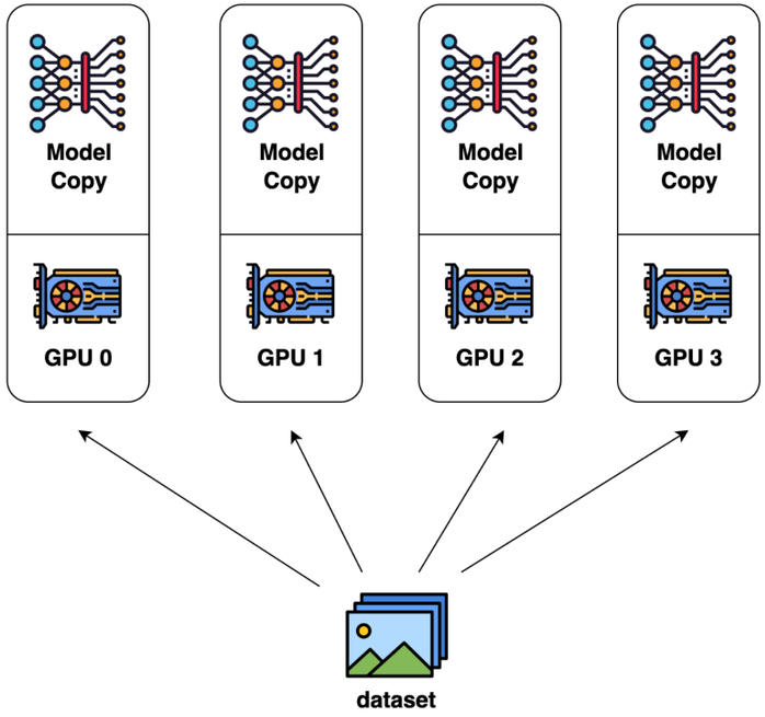
This is the simplest parallelism mechanism. The data is split into several shards, and every shard is allocated to each device, which equals parallel training in the dimension of (data) batch. Every device has an intact copy /replica of the model, and the parameters of the model are updated based on the data split on each device. After back propagation, the gradients will be collected and reduced (like average, sum, max etc) by the parameter server, so that the models on different devices can be synchronized (gradients are distributed and parameters are broadcasted).

A representative realization is Pytorch DDP.

Model parallelism

Having a copy of the model on every GPU device brings about redundancy. Therefore, another parallelism mechanism is model-wise, i.e, the model is split across devices.

Usually, there are two ways to realize it:

• Tensor parallelism: conduct parallel computing within an operation, such as Matrix Multiplication. It split within the transformer layer.
• Pipeline parallelism: conduct parallel computing across layers — split the transformer layers.

left: pipeline parallelism vs right: tensor parallelism

For tensor parallel, we split a tensor along a specific dimension into N parts, with each device holding only 1/N of the entire tensor, while preserving the correctness of the computational graph. This approach requires additional communication to ensure the correctness of the results.

Taking a standard matrix multiplication as an example, suppose we have C = AB. We can split B along its columns into [B₀, B₁, B₂, …, Bₙ], with each device holding one column block. Then, we multiply A with each column block of B on the corresponding device, producing [AB₀, AB₁, AB₂, …, ABₙ]. At this point, each device still holds only part of the result; for example, the device with rank = 0 holds AB₀. To ensure the correctness of the result, we need to gather all the partial results and concatenate them along the column dimension. In this way, we can distribute the tensor across devices while maintaining the correctness of the computation flow.

Typical tensor parallelism implementations include:

• Megatron-LM: 1D tensor parallelism
• Colossal-AI: 2D, 2.5D, and 3D tensor parallelism

For pipeline parallelism, the core idea is to split the model into several segments by layers, with each segment assigned to a different device.

• During the forward pass, each device passes the intermediate activations to the next stage.
• During the backward pass, each device sends the gradients of the input tensor back to the previous pipeline stage.

This approach allows devices to perform computations concurrently, thereby increasing the training throughput.

A notable drawback of pipeline parallel training is that training devices are prone to idle periods, as each stage must wait for the previous stage to complete its computation. This results in wasted computational resources and typically lower acceleration efficiency compared to data parallelism.

Typical implementations of pipeline parallelism include:

• GPipe: basic synchronous pipeline parallelism.
• PipeDream: introduces asynchronous execution and weight stashing.
• PipeDream-2BW: optimizes memory and communication by using two weight buffers (2BW: two-buffer weight).
• PipeDream Flush (1F1B): implements the 1F1B (One Forward, One Backward) scheduling strategy to reduce pipeline bubbles and improve efficiency.

Parallelism for optimizers

As models continue to grow larger, it is becoming increasingly difficult for a single GPU’s memory to accommodate the entire model. Therefore, it is necessary to find ways to optimize memory usage.

Typically, during model training, the GPU needs to store several types of data, including the model parameters, optimizer states, activation outputs, gradients, and some temporary buffers. The proportions of memory consumed by each of these components are shown in the figure below:

It can be observed that model parameters account for only a portion of the total memory consumption during training. When using mixed-precision training, the model states — which include the optimizer states, gradients, and model parameters — take up the majority of the memory. Therefore, it becomes essential to eliminate redundant data stored during the training process.

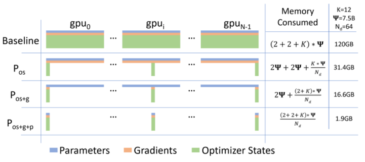
Optimizer state parallelism is one such approach for removing redundant data. The most widely adopted method today is ZeRO (Zero Redundancy Optimizer). ZeRO optimizes the storage of model states by applying sharding, where each GPU holds only 1/N of the model states, meaning that the system maintains only a single copy of the complete model state across all devices.

ZeRO is designed with three optimization stages, each progressively sharding different parts of the model state:

• ZeRO-1: Shards the optimizer states (Optimizer States Sharding).
• ZeRO-2: Shards both optimizer states and gradients (Optimizer States & Gradients Sharding).
• ZeRO-3: Shards the optimizer states, gradients, and model parameters (Optimizer States & Gradients & Parameters Sharding).

Heterogeneous System Parallelism

The methods mentioned above typically require a large number of GPUs to train a large-scale model. However, one often overlooked fact is that CPU memory is much larger than GPU memory. On a typical server, CPUs can easily have hundreds of gigabytes or even terabytes of memory, whereas each GPU usually has only 48 GB or 80 GB of memory. This gap has prompted researchers to rethink why CPU memory is not more widely utilized for distributed training.

Recent advances have explored training large models by leveraging CPU memory or even NVMe storage. The core idea is to offload tensors back to CPU memory or NVMe disks when they are not actively used in computation.

By utilizing a heterogeneous system architecture, it becomes possible to fit a massive model onto a single machine, making large-scale model training more accessible without relying solely on GPU memory.

Multi-Dimensional Hybrid Parallelism

This refers to the combination of various parallelism strategies mentioned above to enable efficient distributed training.

It usually make sense when we conduct full parameters training.

To fully utilize bandwidth, tensor parallelism typically involves the highest communication overhead, while data parallelism and pipeline parallelism require relatively less communication.

Therefore, it is common practice to apply tensor parallelism within a single server, where high-bandwidth interconnects are available, and use data parallelism and pipeline parallelism across servers, where communication bandwidth is more limited.

Automatic parallelism

The multi-dimensional hybrid parallelism approaches mentioned above — such as data parallelism, tensor parallelism, and pipeline parallelism — all require splitting the model across multiple AI accelerator cards. If developers had to implement this manually, it would be extremely challenging, as they would need to carefully balance performance, memory usage, communication overhead, and training effectiveness.

If the model could be automatically partitioned — by operators or by layers — across different accelerators, it would greatly reduce the complexity for developers. This is where automatic parallelism comes into play.

Mixture-of-experts parallelism

Typically, scaling up model size leads to a significant increase in training cost, and limited computational resources become the main bottleneck for training large, dense models. To address this challenge, a deep learning architecture based on sparse Mixture of Experts (MoE) layers was proposed. In this approach, a large model is divided into multiple smaller models (experts), and during each iteration, only a subset of experts is activated based on the input samples, effectively reducing the computational load. A trainable gating mechanism is introduced to control expert selection and ensure sparsity, optimizing overall computation.

By leveraging the MoE architecture, it becomes possible to train ultra-large-scale models with sub-linear increases in computational cost, providing substantial benefits within a fixed computational resource budget. MoE parallelism, in essence, is a form of model parallelism.

The following figure illustrates an example where a model with six experts is trained using two-way expert parallelism: experts 1–3 are placed on the first computing device, and experts 4–6 are placed on the second computing device.