From Brain Scans to Encoding Models: A Beginner’s Guide to fMRI for Machine Learning

Machine learning researchers are increasingly using fMRI data to study how the brain responds to images, videos, language, and other natural stimuli. But before treating brain activity as a prediction target, it is important to understand what fMRI actually measures, how the data is represented, and what it means to predict a brain response.

How the Brain Is Digitized

MRI data represent the brain as a three-dimensional grid of small spatial units called voxels. A voxel is the 3D equivalent of a pixel: while a pixel corresponds to a small location in a 2D image, a voxel corresponds to a small cube in 3D brain space.

In practice, an MRI scanner measures the brain slice by slice. Each slice is a 2D image, and stacking these slices together forms a 3D volume. This volume is not a continuous representation of the brain, but a discretized one: each voxel stores one measured value from a small region of brain tissue.

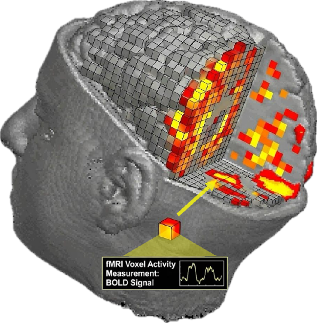
https://home.csulb.edu/~cwallis/482/fmri/fmri.html

Anatomical MRI: High Spatial Resolution

Before talking about brain activity, it is useful to understand anatomical MRI. An anatomical, or structural, MRI scan is designed to capture the physical structure of the brain in high spatial detail.

Compared to fMRI, anatomical MRI is usually acquired at a much higher spatial resolution. A common structural scan may have voxels of about 1 × 1 × 1 mm and takes ~5 minutes for one scan, producing a detailed 3D image of the brain. However, this scan is essentially static: it tells us what the brain looks like, not how its activity changes over time.

Adding Time: Why fMRI Sacrifices Spatial Resolution

Functional MRI extends this voxel-based representation by measuring the brain repeatedly over time. Instead of acquiring one detailed static volume, fMRI acquires a sequence of brain volumes — so we can measure the brain in action.

The time between two consecutive full-brain measurements is called the repetition time, or TR. In many fMRI experiments, the TR is around one to two seconds, meaning that we get a new 3D brain volume every few seconds.

This creates a fundamental tradeoff. To measure activity over time, the scanner must acquire full-brain volumes quickly. As a result, fMRI usually uses larger voxels than anatomical MRI, often around 3 × 3 × 3 mm voxel size.

So while anatomical MRI gives us a high-resolution picture of brain structure, fMRI gives us a lower-resolution but dynamic measurement of brain activity.

This is the basic spatial–temporal tradeoff: smaller voxels require slower scans, while faster scans usually require larger voxels. fMRI prioritizes tracking changes over time rather than capturing fine anatomical detail.

What Does a Voxel Actually Measure?

The brain processes information through the activity of neurons. Neurons communicate using fast electrical signals, often called spikes, which occur on the scale of milliseconds. These signals are the basis of neural computation, but they are not what fMRI measures directly.

fMRI is much slower and much coarser. Each voxel covers a small 3D region of brain tissue, but that region can contain many neurons, blood vessels, glial cells, and other supporting tissue. As a result, the value measured in a voxel is not the activity of a single neuron. It is an aggregate signal from a local population of tissue.

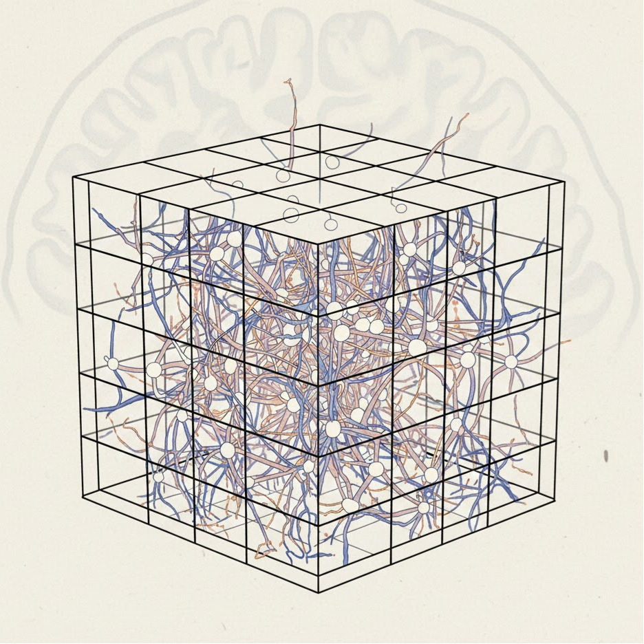
Each fMRI voxel contains many neurons; the measured signal is therefore an aggregate response from a small region of brain tissue, not the activity of a single neuron. Generated using ChatGPT.

What fMRI actually measures is the BOLD signal, short for Blood-Oxygen-Level Dependent signal. When neurons in a region become more active, they consume oxygen. In response, the brain sends more oxygenated blood to that area. This changes the local magnetic properties of the tissue, because oxygenated and deoxygenated blood behave differently in a magnetic field. The MRI scanner detects these changes.

From Raw fMRI to Model-Ready Responses

The BOLD signal does not appear immediately after neural activity. Instead, it follows a delayed response curve called the Hemodynamic Response Function (HRF): the signal rises a few seconds after the stimulus, reaches a peak, and then slowly returns to baseline.

In many fMRI analyses, this delay is modeled using a standard, or canonical, HRF. Rather than using the raw BOLD time series directly, researchers often estimate a response strength for each voxel and each stimulus. This estimated response is usually called beta (β).

Practically, these beta values are often the brain-activity values used in machine learning datasets. Many fMRI datasets publish preprocessed beta responses, where each stimulus is paired with a vector of voxel-wise beta values. In image-to-fMRI encoding models, this is usually the value we try to predict: given an image, predict the beta response it evoked in each voxel.

Before reaching this stage, raw fMRI data must be preprocessed. This usually includes correcting for head motion, aligning functional scans to anatomical MRI, adjusting timing differences between slices, filtering noise, and sometimes normalizing the brain to a common space.

The result is a cleaner, model-ready representation of brain activity: either voxel-wise time series or, more commonly for stimulus-based encoding models, stimulus-level beta responses.

Regions of Interest

A full fMRI response can contain tens of thousands, and sometimes more than 100,000, voxel values. For many research questions, however, we are not equally interested in every voxel in the brain. If we study visual perception, for example, we may care mostly about visual cortex. If we study face processing, we may focus on face-selective regions.

This is where regions of interest, or ROIs, become useful. An ROI is a subset of voxels that are grouped together because they belong to a meaningful anatomical or functional region. Examples include early visual cortex, face-selective regions, body-selective regions, word-selective regions, and scene-selective regions.

For machine learning, ROIs are useful for both practical and interpretability reasons. They reduce the dimensionality of the prediction target, improve the signal-to-noise ratio by focusing on relevant voxels, and make the results easier to interpret. Instead of asking whether a model predicts activity across the entire brain, we can ask a more specific question: how well does it predict activity in a region related to faces, places, words, or visual processing?

In this way, ROIs turn the full voxel space into a more meaningful subspace for analysis.

The Natural Scenes Dataset: Image–fMRI Pairs at Scale

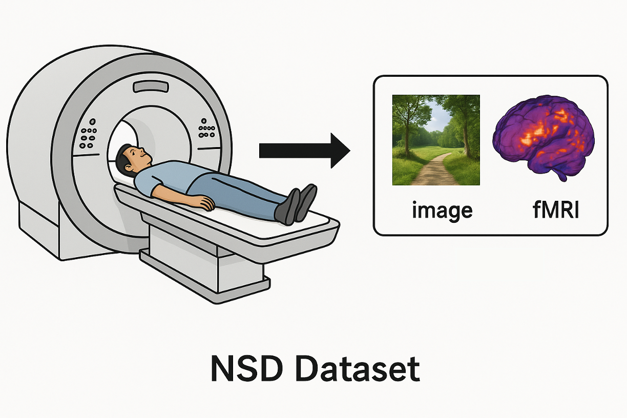
The Natural Scenes Dataset (NSD) is one of the most important datasets for studying how the human brain responds to natural images. In NSD, participants viewed thousands of color natural scenes while their brain activity was recorded with high-resolution 7T fMRI. Here, 7T means 7 Tesla, referring to the magnetic field strength of the scanner. NSD was acquired with whole-brain 7T fMRI at 1.8 mm resolution and 1.6 s TR.

The dataset includes 8 participants, each viewing around 9,000–10,000 distinct natural images over 30–40 scan sessions. Across repeated presentations, this corresponds to roughly 22,500–30,000 trials per participant.

The useful structure of NSD is that it connects each image to the fMRI response it evoked in a specific subject. After preprocessing, these responses are often represented as voxel-wise beta values: for each image, we get a vector of estimated activity values across voxels. This creates a practical dataset of paired examples: image → voxel-wise fMRI response.

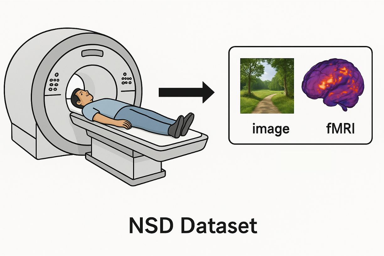
Generated using ChatGPT.

NSD also provides ROI masks, which allow researchers to focus on specific brain regions instead of using all voxels. These masks may come from anatomical definitions or from functional localizer experiments, where subjects view categories such as faces, bodies, places, or words. Voxels that respond more strongly to a category can be grouped into a corresponding ROI, producing subject-specific masks for meaningful brain regions.

Encoding Models

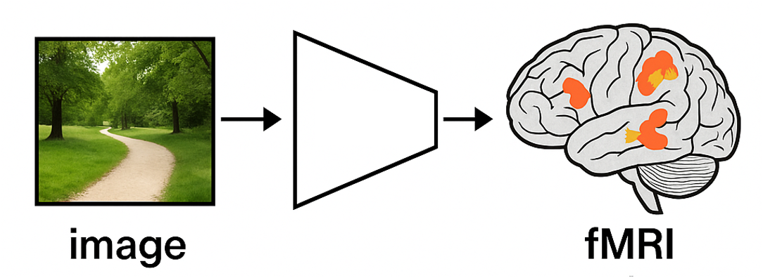
An encoding model learns to predict brain activity from an external stimulus. In the visual setting, the input is usually an image, and the output is the fMRI response evoked by that image.

After preprocessing, this response is often represented as a vector of voxel-wise beta values. So the learning problem can be written simply as: image → predicted voxel responses

Generated using ChatGPT.

CLIP2Brain: A Modern Encoding Model

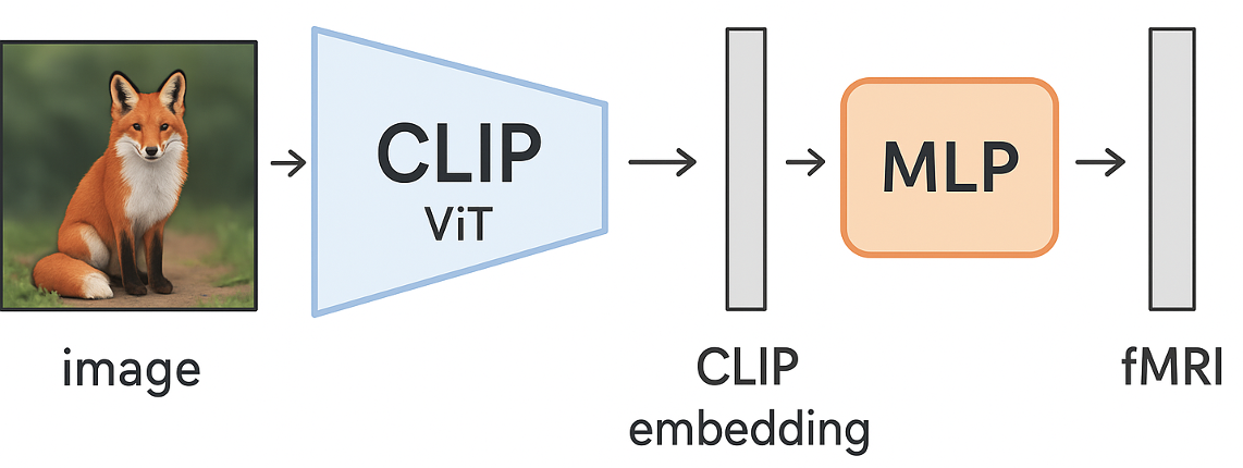
A modern example of an image-to-fMRI encoding model is **CLIP2Brain**. The main idea is to use representations from a pretrained vision-language model, such as CLIP, as features for predicting brain activity.

Instead of training an image encoder from scratch, CLIP2Brain passes each image through a pretrained CLIP vision model. This produces a high-level image embedding, which is then mapped to voxel-wise fMRI responses using a simple prediction head, such as a linear layer or a small MLP.

The pipeline is: image → CLIP image embedding → prediction head → fMRI response

In this setup, the CLIP image encoder is kept frozen and used only as a feature extractor. The part trained on fMRI data is the prediction head, which learns the mapping from CLIP embeddings to brain responses. The CLIP2Brain paper explores several design choices, including different CLIP backbones, dataset sizes, and prediction-head architectures. A main finding is that CLIP-based visual representations show strong alignment with brain responses, suggesting that features learned by modern vision-language models are useful for predicting activity in the human visual cortex.

Generated using ChatGPT.

TRIBE v2: Extending Encoding Models to Video, Audio, and Text

While CLIP2Brain focuses on static images, many real-world experiences are dynamic and multimodal. A movie, for example, contains visual motion, sound, spoken language, and temporal context. TRIBE v2 extends the encoding-model idea to this more natural setting by predicting fMRI responses from video, audio, and text. The released model combines feature extractors for text, video, and audio into a unified Transformer architecture that maps multimodal representations onto the cortical surface.

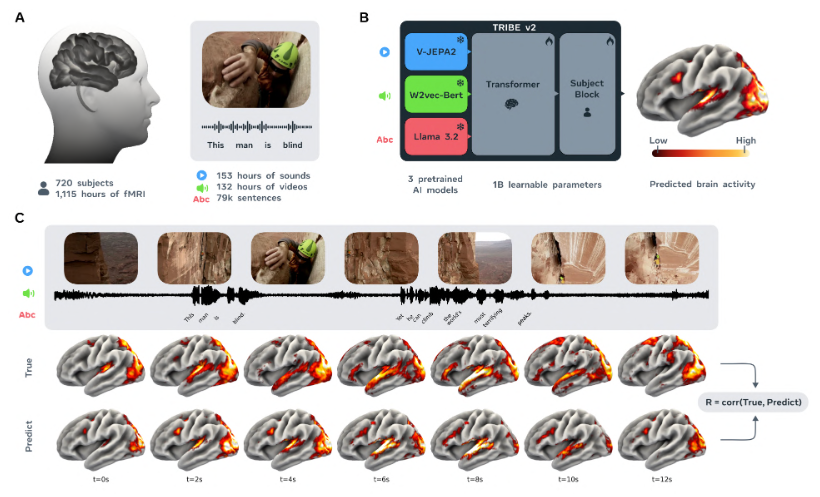
From TribeV2’s paper.

Conceptually, the difference is simple: CLIP2Brain asks how the brain responds to an image, while TRIBE v2 asks how the brain responds to a temporally evolving stimulus. Instead of producing one response per image, TRIBE v2 predicts a sequence of brain responses over time. In the released model, predictions are for an “average” subject and are represented on the fsaverage5 cortical mesh, with around 20k vertices.

This makes TRIBE v2 especially interesting for studying naturalistic perception. The paper presents TRIBE v2 as a tri-modal foundation model of vision, audition, and language, trained on a unified dataset of over 1,000 hours of fMRI across 720 subjects.

Possible pipeline sentence: video / audio / text → modality-specific features → temporal Transformer → predicted fMRI response

Evaluating Encoding Models

After training an encoding model, we need to compare its predicted brain responses with the measured fMRI responses on held-out data. The most common evaluation is done voxel by voxel, or ROI by ROI: for each voxel, we compare the predicted response across test stimuli to the measured response across the same stimuli.

A common metric is Pearson correlation. It measures whether the predicted and measured responses vary together across stimuli. This is useful because it focuses on the shape of the response pattern and is less sensitive to scale differences.

Another common metric is R², or coefficient of determination. R² measures how much variance in the measured response is explained by the model. Unlike correlation, it is sensitive to scale and bias, so a model can have good correlation but worse R² if its predictions are systematically too large, too small, or shifted.

One important concept in fMRI evaluation is the noise ceiling. fMRI measurements are noisy, and even repeated presentations of the same stimulus do not produce exactly identical responses. Because of this, there is an upper bound on how well any model can predict the measured data. The noise ceiling estimates this upper bound, often using response reliability across repeated trials or subjects.

This means that a numerically “low” score is not always a bad result. If the model approaches the noise ceiling, it may already be close to the best performance possible given the noise in the data. For this reason, encoding-model performance should be interpreted relative to the reliability of the measured fMRI responses, not only by the raw metric value.

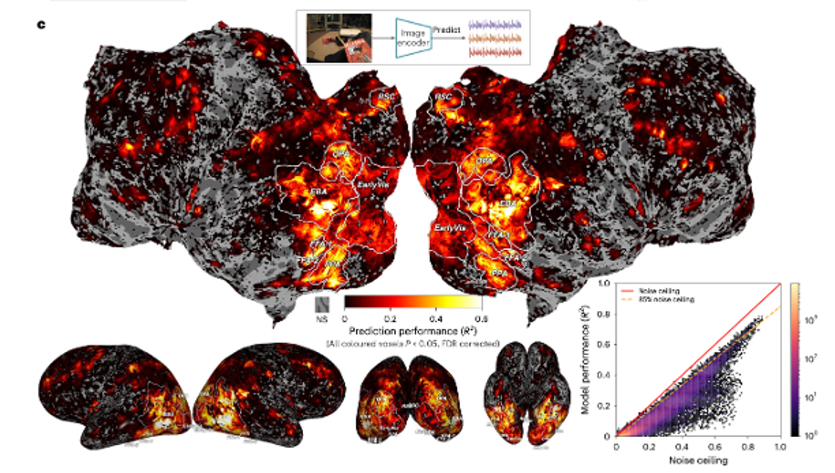
From Clip2Brain’s paper.

Conclusion

fMRI data gives us a fascinating way to study how the brain responds to natural stimuli, but it is important to remember what this data really represents. It is not a direct recording of individual neurons, but a voxel-wise, indirect, and noisy measurement of brain activity through the BOLD signal. After preprocessing, this signal can be transformed into practical targets for machine learning, such as voxel-wise beta values or ROI-level responses.

Encoding models build on this representation by learning mappings from stimuli — images, videos, audio, or text — to predicted brain responses. Models such as CLIP2Brain show how pretrained visual representations can be used to predict responses to images, while models such as TRIBE v2 extend this idea to richer, naturalistic, multimodal stimuli.

This blog is meant to be a high-level quick start for ML researchers who want to begin working with fMRI data. Many important details are simplified here, including MRI physics, preprocessing pipelines, statistical modeling, ROI definitions, and evaluation protocols. The goal is not to cover the entire field, but to build the basic mental model needed to understand image-to-fMRI and multimodal encoding models.

Personally, I am very passionate about this research direction, especially the connection between generative models and brain activity. I am particularly interested in generating stimuli, or optimizing images and videos, to maximize predicted activity in specific brain regions or ROIs. I believe this direction can become a powerful tool for studying what different brain regions represent and how modern machine learning models can help us explore brain function.

Feel free to reach out:)