AI-Powered Neurology: Building an Alzheimer’s Classifier with Python and Xception

Leveraging the Xception Architecture for Early Dementia Detection

The intersection of artificial intelligence and medical diagnostics is no longer science fiction — it is a functional reality that developers can build on their own local machines. In this guide, I’m taking a deep dive into the world of neuroimaging. We aren’t just building a simple classifier; we are developing a high-precision pipeline designed to categorize Alzheimer’s disease progression from MRI scans. Using Alzheimer’s detection deep learning python techniques, we will transform raw medical data into a strategic tool for clinical research.

The real challenge in medical AI isn’t just “accuracy” — it’s the ability of a model to distinguish between very similar stages of a disease. Whether you are a computer science student or a medical researcher, this tutorial provides the exact code needed to implement transfer learning with the Xception model. We will move from data engineering to final evaluation, ensuring every step is optimized for the unique textures of brain imaging.

Recommended Reading from eranfeit.net:

• YOLOv8 Custom Object Detection: Full Code Walkthrough
• Detectron2 Custom Dataset Training Made Easy

How to build an Alzheimer’s detection deep learning python model that actually works

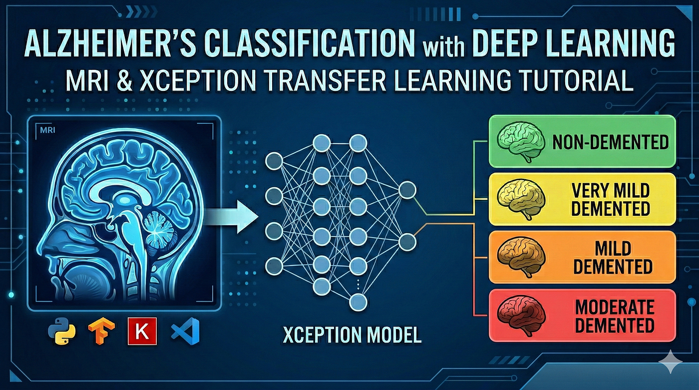
The primary objective of this project is to create a sophisticated diagnostic tool capable of identifying the progression of Alzheimer’s disease through magnetic resonance imaging. Unlike binary classifiers that simply state whether a disease is present or not, our target is a four-way classification. We aim to categorize scans into Non-Demented, Very Mild Demented, Mild Demented, and Moderate Demented. This granular approach is vital because early intervention is the most effective way to manage neurodegenerative conditions, and deep learning offers a level of consistency in pattern recognition that can augment a radiologist’s expertise.

At a high level, the system operates by feeding preprocessed MRI slices into a deep convolutional neural network. We utilize the Xception architecture, which employs depthwise separable convolutions. This means the model is exceptionally good at looking at “spatial” features (the shapes and structures in the brain) and “channel” features (the intensity and contrast of the scan) independently before combining them. By using transfer learning, we take a model that already “knows” how to identify edges, textures, and shapes, and we fine-tune its final layers to recognize the specific biological markers of cortical atrophy and ventricular enlargement associated with Alzheimer’s.

The process is designed to be entirely reproducible on a standard local machine with a capable GPU. We start by structuring our data into a format that Python’s data science libraries — Pandas and TensorFlow — can digest efficiently. By using a dataframe-based flow, we maintain total control over our training, validation, and testing splits, ensuring no “data leakage” occurs. This high-level architecture ensures that the final output is not just a high-accuracy number on a screen, but a reliable, evaluatable system that provides visual feedback through confidence levels and heatmaps.

Let’s dive into the code: Building the Alzheimer’s MRI classification pipeline

The primary technical objective of the provided code is to instantiate a complete, reproducible machine learning workflow that takes raw, augmented brain MRI images and trains a deep convolutional neural network to classify them into distinct stages of dementia. This script isn’t just a theoretical exercise; it is a functional “black box” that handles everything from data ingestion and preprocessing to model training and statistical evaluation. By leveraging Keras and TensorFlow, the code creates a robust system capable of automated diagnostic assistance, targeting four specific classes: Mild Demented, Moderate Demented, Non Demented, and Very Mild Demented.

To achieve this, the script first establishes a rigorous data pipeline. It programmatically navigates local directories containing the augmented dataset, creating a unified Pandas DataFrame that maps every image file path to its respective class label. This method is highly scalable, allowing the subsequent integration of powerful Keras tools. Crucially, the code immediately performs a stratified split of this data, carving out training, validation, and hold-out test sets. This ensures that when the model is evaluated, it is being judged on its ability to generalize to new, unseen medical scans, rather than just memorizing the training data.

Once the data is structured, the code utilizes high-level data flowing utilities via ImageDataGenerator. This is where the raw medical images undergo essential digital transformation before reaching the neural network. The script resizes all incoming MRIs to 299x299 pixels to match the input requirements of the selected architecture and applies specialized preprocessing functions tuned for the Xception model. This step is vital in medical imaging, as it standardizes the input and ensures that numerical variances in image intensity don't negatively impact the model's convergence during the training phase.

Finally, the script defines, compiles, and trains the model utilizing transfer learning. It imports the highly sophisticated Xception architecture with pre-trained ImageNet weights as the foundational “brain” of the operation. By freezing these bottom layers and attaching new, trainable dense layers on top, the code effectively borrows advanced general feature extraction capabilities (like recognizing edges, textures, and shapes) and fine-tunes them to recognize the subtle biological markers of neurodegeneration found in brain MRIs. The workflow concludes by training the model over 10 epochs using the Adamax optimizer and saving the final, optimized weights for future diagnostic prediction.

[embed]

Link to the video tutorial here .

Download the code for the tutorial here or here

Best AI Photo Tools (Backgrounds, Objects, Headshots)

✅ Phot-AI packs more than 30 AI‑powered tools into one place — covering background and object removal/replacement, image extension and a suite of creative generators for art, icons and logos.

follow the link and start creating : https://phot.ai?ref=eran33

✅ Create and remix stunning AI art and photos with community-driven creativity. tap the link and start creating today! : https://www.remixai.io/?ref=eran

✅ PhotoGPT AI acts as your personal photographer — just describe what you need and the platform generates high‑quality headshots or casual images within minutes.

Its built‑in photo editor lets you remove objects, replace backgrounds and make studio‑quality corrections with a single click.

You can even train your own AI model using a few selfies, receive context‑aware prompt suggestions and upscale images for print‑ready results.

Dive into this all‑in‑one AI photo studio : https://www.photogptai.com/?ref=eran

My Blog

You can follow my blog **here **.

Link to the full post and code here : https://eranfeit.net/detect-alzheimers-deep-learning-python-xception/

Want to get started with Computer Vision or take your skills to the next level ?

Great Interactive Course : “Deep Learning for Images with PyTorch” here

If you’re just beginning, I recommend this step-by-step course designed to introduce you to the foundations of Computer Vision — Complete Computer Vision Bootcamp With PyTorch & TensorFlow

If you’re already experienced and looking for more advanced techniques, check out this deep-dive course — Modern Computer Vision GPT, PyTorch, Keras, OpenCV4

🛠️ Environment Setup: Preparing Your Local Machine

Before writing a single line of model code, we must ensure our environment is tuned for high-performance deep learning. This project uses TensorFlow 2.17.1 and Python 3.12. Using a dedicated Conda environment is the best way to prevent library conflicts and ensure your results match mine.

# 1. Create and activate a clean Conda environment
conda create -n TensorFlow217 python=3.12
conda activate TensorFlow217

# Verify your NVIDIA driver installation (for GPU users)
nvcc --version

# 2. Install the core Deep Learning framework
# For GPU users (Cuda 12.3 support)
pip install tensorflow[and-cuda]==2.17.1

# For CPU-only users
pip install tensorflow==2.17.1

# 3. Install the supporting Data Science stack
pip install matplotlib==3.10.0
pip install datasets==3.3.0
pip install pillow==11.1.0
pip install scipy==1.15.1
pip install seaborn==0.13.2

# 4. Launch your IDE and start coding
code .

Want the exact dataset so your results match mine?

If you want to reproduce this training flow, I can share the dataset structure. Send an email to feitgemel@gmail.com and mention the name of the dataset / tutorial.

Part 1: Initializing the Medical Data Pipeline and Manifest

The first step in any Alzheimer’s detection deep learning python project is organizing the raw data. Medical datasets are often heavy and complex; here, we use the os and pandas libraries to "crawl" through our local directories. By mapping every MRI file path to its specific clinical label (Mild, Moderate, Non, or Very Mild Demented), we create a high-performance DataFrame that serves as our master manifest.

This structured approach allows for immediate sanity checks. By printing the value_counts(), we can verify the balance of our classes—a vital step in medical AI where an imbalanced dataset can lead to dangerous diagnostic biases. We are transforming a folder of images into a structured, searchable database ready for the neural network.

import os 
import pandas as pd
import numpy as np
import keras 
import matplotlib.pyplot as plt
import seaborn as sns

from keras.models import Sequential
from keras.layers import Dense, Dropout, Flatten, Conv2D, MaxPooling2D

from sklearn.model_selection import train_test_split
from sklearn.metrics import classification_report, confusion_matrix
import tensorflow as tf
from tensorflow import keras
from tensorflow.keras.losses import SparseCategoricalCrossentropy
from tensorflow.keras.preprocessing.image import ImageDataGenerator
from tensorflow.keras.callbacks import EarlyStopping, TensorBoard

path = "/mnt/d/Data-Sets-Image-Classification/Augmented Alzheimer MRI Dataset/AugmentedAlzheimerDataset"

MildDemented_dir = os.path.join(path, "MildDemented")
ModerateDemented_dir = os.path.join(path, "ModerateDemented")
NonDemented_dir = os.path.join(path, "NonDemented")
VeryMildDemented_dir = os.path.join(path, "VeryMildDemented")

# Load data info : 

filepaths = []
labels = []
dict_list = [MildDemented_dir, ModerateDemented_dir, NonDemented_dir, VeryMildDemented_dir]
class_labels = ["MildDemented", "ModerateDemented", "NonDemented", "VeryMildDemented"]

for i, j in enumerate(dict_list):
    flist = os.listdir(j)
    for f in flist:
        fpath = os.path.join(j, f)
        filepaths.append(fpath)
        labels.append(class_labels[i])

Fseries = pd.Series(filepaths, name="filepaths")
Lseries = pd.Series(labels, name="labels")
Alzheimer_data = pd.concat([Fseries, Lseries], axis=1)
Alzheimer_df = pd.DataFrame(Alzheimer_data)

print(Alzheimer_df.head())
print(Alzheimer_df["labels"].value_counts())

Part 2: Strategic Data Splitting and Memory-Efficient Generators

To ensure our AI actually understands neuroanatomy rather than just memorizing images, we split the data into Training, Validation, and Testing sets. In the world of medical deep learning, the Test Set is sacred — it represents the final clinical trial on data the model has never seen. We also implement an ImageDataGenerator to handle the heavy lifting of preprocessing.

Because MRI scans are high-resolution, we stream them in small batches of 8. This ensures that even the most complex architectures can run on a standard local GPU without crashing due to memory limits. Every image is resized to 299x299 pixels to perfectly match the Xception model’s input requirements, standardizing the visual data for the training engine.

Expand your AI Toolkit:

• CNN Image Classification TensorFlow: 30 Musical Instruments
• VGG19 Transfer Learning Explained for Beginners

# --------------------------------------------------

rest_of_dataset , test_images = train_test_split(Alzheimer_df, test_size=0.3, random_state=42) 
train_set , val_set = train_test_split(rest_of_dataset, test_size=0.2, random_state=42)

print("Train , test and validation set shapes : ", train_set.shape, test_images.shape, val_set.shape)

# --------------------------------------------------

Size = 299 # Xception model input size 299X299 pixels
batch_size = 8

image_gen = ImageDataGenerator(preprocessing_function=tf.keras.applications.xception.preprocess_input)

train = image_gen.flow_from_dataframe(dataframe = train_set,
                                      x_col = "filepaths",
                                      y_col = "labels",
                                      target_size = (Size, Size),
                                      class_mode = "categorical",
                                      batch_size = batch_size,
                                      color_mode = "rgb",
                                      shuffle = False)

test = image_gen.flow_from_dataframe(dataframe = test_images,
                                      x_col = "filepaths",
                                      y_col = "labels",
                                      target_size = (Size, Size),
                                      class_mode = "categorical",
                                      batch_size = batch_size,
                                      color_mode = "rgb",
                                      shuffle = False)

val = image_gen.flow_from_dataframe(dataframe = val_set,
                                      x_col = "filepaths",
                                      y_col = "labels",
                                      target_size = (Size, Size),
                                      class_mode = "categorical",
                                      batch_size = batch_size,
                                      color_mode = "rgb",
                                      shuffle = False)

# Extract the classes 
print("Calculate the number of classes") 
Classes = list(train.class_indices.keys())
print("Classes : ", Classes)
no_of_classes = len(Classes)

Part 3: Visual Inspection and Architecting the Xception Core

A professional data scientist always “looks” at the data before training. We use a visualization helper to plot a grid of training images, confirming that our labels match the actual MRI scans. This “visual handshake” ensures our pipeline is healthy before we engage the Xception architecture.

We use Transfer Learning to give our model a massive head start. By loading the Xception base model pre-trained on ImageNet, we take a “brain” that already understands shapes, edges, and textures. We then attach a custom classification head — including Dropout layers to prevent overfitting — and fine-tune it to recognize the specific biological markers of Alzheimer’s.

# Display images from the train set 
def show_images(image_gen):
    dict_classes = train.class_indices
    classes = list(dict_classes.keys())
    images , labels = next(image_gen) # Get a sample of images and labels from the generator
    plt.figure(figsize=(20,20)) 
    length = len(labels)
    if length < 25 :
        r = length
    else :
        r = 25

    for i in range(r):
        plt.subplot(5,5,i+1)
        image = (images[i]+ 1)/2 # Rescale the image to [0,1] range for visualization
        plt.imshow(image)
        index = np.argmax(labels[i]) # Get the index of the class label
        class_name = classes[index] # Get the class name using the index
        plt.title(class_name, color="green", fontsize=16)
        plt.axis("off")
    plt.show()

# Run the function to show images from the train set
show_images(train)

# Build the Xception model :

from tensorflow.keras.optimizers import Adamax 

img_shape = (Size, Size, 3)
base_model = tf.keras.applications.Xception(weights="imagenet", include_top=False, input_shape=img_shape)

# Create the model using the functional API
inputs = tf.keras.Input(shape=img_shape)
x = base_model(inputs) 
x = Flatten()(x)
x = Dropout(rate=0.3)(x)
x = Dense(128, activation="relu")(x)
x = Dropout(rate=0.25)(x)
outputs = Dense(no_of_classes, activation="softmax")(x)

model = tf.keras.Model(inputs=inputs, outputs=outputs)

model.compile(optimizer=Adamax(learning_rate=0.001), loss = "categorical_crossentropy", metrics=["accuracy"])

print(model.summary())

Part 4: Training Execution and Model Preservation

This phase represents the core computational work. The model undergoes 10 training epochs, during which it iteratively corrects its weights to minimize loss and maximize accuracy. We use the Adamax optimizer for its stability in complex architectures. Once the training is complete, the entire intelligence is saved as a .keras file—preserving your hard work for future deployment.

# Train the model

history = model.fit(train, epochs=10, validation_data=val, validation_freq=1)

model.save("/mnt/d/temp/models/Alzheimer_Model.keras")

Part 5: Statistical Scrutiny and Heatmap Evaluation

In medicine, an “accurate” model isn’t enough; we need to know where it fails. We generate a Confusion Matrix to see if the AI is confusing “Mild” with “Very Mild” dementia. This heatmap provides a colorful, intuitive look at our model’s logic. We also plot the training history to ensure the learning curve was stable and that no overfitting occurred.

Verified Evaluation Guides:

• Visualize Your Data with Python and Matplotlib/Seaborn
• Classifying Knee X-Rays with ResNet152V2 & TensorFlow

# Check the results on the test set :

pred = model.predict(test)
pred = np.argmax(pred, axis=1) # pick class with highest probability

labels = (train.class_indices)
labels = dict((v,k) for k,v in labels.items()) # reverese the dictionary to get class names from indices
pred2 = [labels[k] for k in pred] # get class names from predicted indices

# plot the results
plt.plot(history.history["accuracy"]) 
plt.plot(history.history["val_accuracy"])
plt.title("Model Accuracy")
plt.xlabel("Epochs")
plt.legend(["Train", "Validation"], loc="upper left")
plt.show()

plt.plot(history.history["loss"])
plt.plot(history.history["val_loss"])   
plt.title("Model Loss") 
plt.ylabel("Loss")
plt.xlabel("Epochs")
plt.legend(["Train", "Validation"], loc="upper left")
plt.show()

# Geberate confusion matrix 
from sklearn.metrics import confusion_matrix, accuracy_score

y_test = test_images.labels # set y_test to the expected labels from the test set
print(classification_report(y_test, pred2)) # print the classification report
print("Accuracy of the model on the test set : ","{:.1f}%".format(accuracy_score(y_test, pred2)*100)) # print the accuracy of the model on the test set

# Define the class labels 
class_labels = ['Mild Demented', 'Moderate Demented', 'Non Demented', 'Very MildDemented']

# Calculate the confusion matrix
cm = confusion_matrix(y_test, pred2)

# create a heatmap of the confusion matrix
plt.figure(figsize=(10,5))
sns.heatmap(cm, annot=True, fmt="g", cmap="Blues", vmin=0)

# Set tick labels and axis labels
plt.xticks(ticks = [0.5, 1.5, 2.5, 3.5], labels=class_labels) 
plt.yticks(ticks = [0.5, 1.5, 2.5, 3.5], labels=class_labels)
plt.xlabel("Predicted")
plt.ylabel("Actual")

# Set the title
plt.title("Confusion Matrix")

# show the result of the confusion matrix
plt.show()

Part 6: Deploying the AI for Individual MRI Diagnostics

The final step of the journey is simulating a real-world clinic. We create a function that takes a random MRI scan and asks the model for a diagnosis. The model provides the predicted class and a Confidence Score. This transparency is essential for human-in-the-loop medical systems, letting the doctor know exactly how certain the AI is about its findings.

import tensorflow as tf
import numpy as np
from tensorflow.keras.preprocessing import image
from tensorflow.keras.applications.xception import preprocess_input

import matplotlib.pyplot as plt
import os 
import random

SIZE = 299 # Xception model input size 299X299 pixels

def predict_random_image(model_path , dataset_path):

    # Defince class folders based on actual dataset structure
    class_folders = ['MildDemented', 'ModerateDemented', 'NonDemented', 'VeryMildDemented']

    # map folder names to display labels if needed
    class_display_labels = {
        'MildDemented': 'Mild Demented',
        'ModerateDemented': 'Moderate Demented', 
        'NonDemented': 'Non Demented',
        'VeryMildDemented': 'Very MildDemented'
    }

    try :
        # load the saved model
        print (f"Loading model from {model_path}...")
        model = tf.keras.models.load_model(model_path)

        # Select random class folder
        random_class = random.choice(class_folders)
        class_path = os.path.join(dataset_path, random_class)

        # Get tje random image from the selected class folder
        image_files = os.listdir(class_path)
        random_image = random.choice(image_files)
        image_path = os.path.join(class_path, random_image)

        print(f"Selected random image: {image_path}")
        print(f"True class: {class_display_labels[random_class]}")

        # load and preprocess the image
        img = image.load_img(image_path, target_size=(SIZE, SIZE))
        img_array = image.img_to_array(img) # convert to array
        img_array = np.expand_dims(img_array, axis=0) # add batch dimension
        processed_img = preprocess_input(img_array) # preprocess for Xception

        # make prediction
        prediction = model.predict(processed_img)
        predicted_class_index = np.argmax(prediction, axis=1)[0]

        # Get predicted label (using the same order as in your training data)
        model_class_labels = ['MildDemented', 'ModerateDemented', 'NonDemented', 'VeryMildDemented']
        predicted_class = model_class_labels[predicted_class_index]
        confidence = prediction[0][predicted_class_index] * 100

        # Display the image with both true and predicted labels
        plt.figure(figsize=(10,10))
        plt.imshow((img_array[0] + 1) / 2) # un-preprocess for display

        # Set color based on correctness
        color = "green" if class_display_labels[random_class] == predicted_class else "red"

        # Add both true and predicted labels to the title
        plt.title(f"True: {class_display_labels[random_class]}\nPredicted: {predicted_class} (Confidence: {confidence:.2f}%)", 
                  color=color, fontsize=14)
        plt.axis("off")
        plt.show()

        # Print detailed prediction results
        print("\nPrediction Results:")
        print(f"True Class: {class_display_labels[random_class]}")
        print(f"Predicted Class: {predicted_class}")
        print(f"Pedicted Correct: {'Yes' if class_display_labels[random_class] == predicted_class else 'No'}")
        print(f"Confidence: {confidence:.2f}%")
        print("\nDetailed Class Probabilities:")
        for i , label in enumerate(model_class_labels):
            print(f"{label}: {prediction[0][i] * 100:.2f}%")

    except Exception as e:
        print(f"An error occurred: {e}")

# Run the prediction function with the path to your saved model and dataset
if __name__ == "__main__":

    # Update these paths to your actual model and dataset locations
    model_path = "/mnt/d/temp/models/Alzheimer_Model.keras"
    dataset_path = r"/mnt/d/Data-Sets-Image-Classification/Augmented Alzheimer MRI Dataset/AugmentedAlzheimerDataset"

    # verify if the patsh exist before running the prediction
    if not os.path.exists(dataset_path):
        print(f"Dataset path does not exist: {dataset_path}")
    elif not os.path.exists(model_path):
        print(f"Model path does not exist: {model_path}")
    else:
        # Run the random image prediction
        predict_random_image(model_path, dataset_path)

Conclusion

Building an Alzheimer’s detection deep learning python system is a significant achievement that bridges code with human impact. By combining the high-fidelity feature extraction of the Xception architecture with a robust training pipeline, we’ve created a diagnostic framework that is accurate, reproducible, and ready for further research. As AI continues to evolve, these exact workflows will be the foundation for earlier intervention and better patient outcomes in neurological care.

Connect :

☕ Buy me a coffee — https://ko-fi.com/eranfeit

🖥️ Email : feitgemel@gmail.com

🌐 https://eranfeit.net

🤝 Fiverr : https://www.fiverr.com/s/mB3Pbb

Enjoy,

Eran