Can two identical-looking drugs actually be different? I ran the numbers to find out

(Z vs T, CLT, confidence intervals, hypothesis testing) into one real example.

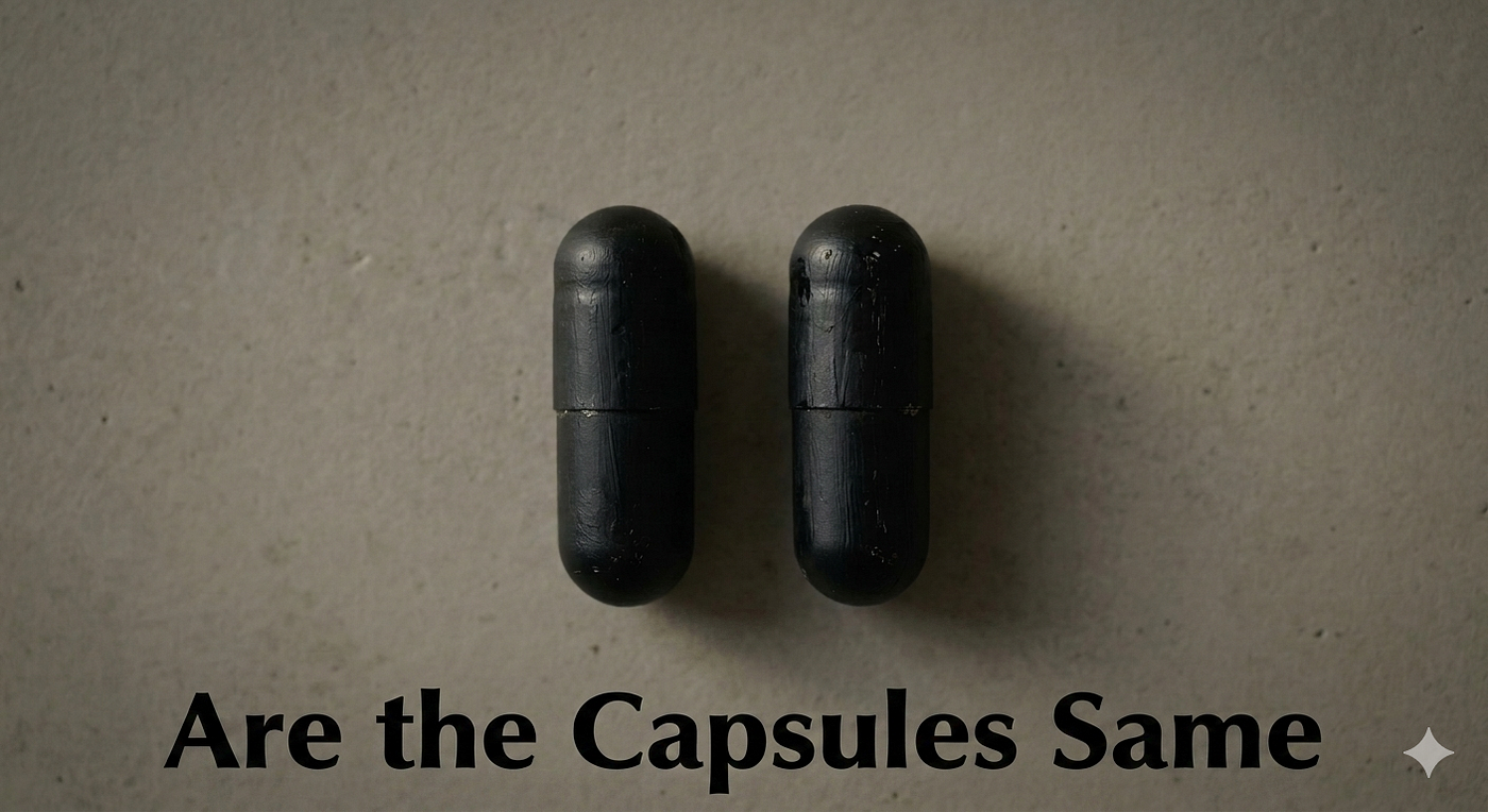
A few nights ago, deep in stats revision, a thought hit me: if someone handed you two identical-looking pills, no labels, no smell difference, could you actually prove they’re different just from how people react to them? Turns out yes, and walking through it with made-up data is what finally made hypothesis testing click for me.

Setup: two unlabeled drugs, X and Y. Give X to ten people with headaches, Y to a different ten, and time how many minutes until the headache goes away.

Because each patient gets only one drug (not both), this is an independent two-sample test, not a paired test. And because we don’t know the true population standard deviation of either drug’s effect (we only have sample data), we must use a t-statistic, not a Z-statistic — exactly the distinction you just learned.

The Hypotheses:

H₀ (null): μₓ = μᵥ —the two drugs have the same true average effect (despite looking different on paper, they’re statistically indistinguishable)

H₁ (alternative): μₓ ≠ μᵥ — the drugs have genuinely different average effects

The data (drafted as a realistic sample — time to relief, in minutes)

Our Data

Intuition: X averages 22.6 minutes, Y averages 28.2. A 5.6-minute gap. But people heal at different rates regardless of the pill, so that gap alone proves nothing, it could easily be noise. That’s the actual question a hypothesis test answers.

We start by assuming the drugs are identical (the null hypothesis), then ask: how likely is a gap this big purely by chance?

Why a t-test, not a z-test? Because we don’t know the true population variability, we’re estimating it from these small samples. Smaller sample, more uncertainty, so the t-distribution adds slightly fatter tails to account for that.

Drug X (n₁ = 10): 22, 25, 19, 24, 21, 23, 20, 26, 22, 24 x̄₁ = 22.6, s₁ ≈ 2.22

Drug Y (n₂ = 10): 27, 30, 26, 29, 31, 28, 25, 30, 29, 27 x̄₂ = 28.2, s₂ ≈ 1.93

THE TWO APPROACHES

Here , Welch–Satterthwaite equation is:

We will use APPROACH 1 : POOLED (STUDENTS ) t-test for our problem and assume or required to have two groups off sample with same true variance The Maths behind: spread within X is about 2.22 minutes, within Y about 1.93. Combine those into a standard error of roughly 0.93 minutes. Divide the 5.6-minute gap by that, and the t-value comes out to −6.01

Degree Of Freedom:

• Degrees of freedom is just “how many numbers are actually free to be anything”
• Since we have got 10 numbers as data points and we already know their average. If we pick randomly any 9 of them, then the 10th one isn’t free anymore, it is restricted to be something which make up to true mean. So out of 10 numbers, only 9 are truly “free.”
• That’s where n − 1 comes from.
• Now do that for two separate groups. Each group loses one degree of freedom to its own mean, so you just add them up: (n₁ − 1) + (n₂ − 1), or n₁ + n₂ − 2. With 10 people per group, that’s 9 + 9 = 18.

Pooled Variance:

Combining both groups’ spread into one number The formula, in words: take each group’s variance, weight it by how many “free” data points it had (n−1, the degrees of freedom from before), add those together, then divide by the total degrees of freedom.

With our actual numbers: Group X: variance s₁² ≈ 4.93, with 9 degrees of freedom Group Y: variance s₂² ≈ 3.73, with 9 degrees of freedom Pooled variance =(9 × 4.93 + 9 × 3.73) / 18 = (44.4 + 33.6) / 18 = 78 / 18 = 4.33 Pooled Standard Deviation (sₚ) = square root of pooled variance =√4.33 ≈ 2.08

Standard Error ( S.E. ) :

• It is the measures the spread of group average or mean from the true mean
• if I tested 10 random people on a drug, how much could that group’s average wobble around
• If I grabbed a totally different random batch of 10 people and gave them the exact same drug, their average wouldn’t land on exactly 22.6 minutes again, it’d be somewhere close, but wobbling a bit. Standard error is just a number for how much that wobble usually is

S.E.=2.08 × √0.2 ≈ 0.93 Here, that wobble comes out to about 0.93 minutes.

t- Statistics:

• T-Test is a statistics method to determine significance changes between means of two groups. It helps us to determine whether the data sets belong to the same group or not. This comparison is often called a T-test.
• It tells us how many standard errors fit into the gap between between the hypothesized population mean and your calculated sample mean

x̄ = Sample mean μ = Population mean (under the null hypothesis) SE=Standard Error

t= (22.6 − 28.2) / 0.93 ≈ −6.01 Here it comes out to about 6.01. The gap isn’t one typical wobble away, it’s six of them stacked end to end

Critical Value:

• In plain terms, is the line in the threshold .
• For my test, with 18 degrees of freedom and the usual 5% cutoff, that line sits at ±2.101.
• Cross it, either direction, and you’re officially too far from zero to blame on chance. My t-value of −6.01 isn’t just past that line, it’s nearly three times past it.

Critical value: t_crit(α = 0.05, two-tailed, df = 18) = 2.101

P-value:

• It answer to “What is the chance we would still see the result this big purely by luck ” assuming the null hypothesis is true
• p-value measures the probability of getting results as extreme or more extreme than what you observed , instead of keeping in a binary conclusion of yes/no
• It gives us the likelihood of chances in range of [0,1]
• Our t-statistics value was 6.01 (ignoring sign). That’s a big value, even the most extreme α=0.0005 has 3.922 t-statistics value, which corresponds to a one-tail probability of just 0.0005 (or 0.001 two-tailed).
• p < 0.001. That’s literally as far as the table can take you. It can’t tell you the result is 0.00001 specifically(we will see in code)
• To get an exact number beyond that bound, you need software that actually integrates the t-distributions' curve, things like Excel’s T.DIST function, Python's scipy.stats.t.sf(), R's pt(), or any online t-distribution calculator. That's where a precise figure like 0.00001 (or whatever the exact computed value is) actually comes from, not from reading a t-score table .
• p-value = 0.00001

Together they say the same thing two ways: critical value marks where the line is, p-value tells you exactly how far past it you landed.

Confidence interval :

A confidence interval is a range of plausible values for a population parameter, computed from your sample. The correct interpretation of a 95% CI is: if we repeated this sampling and Cl procedure many times, about 95% of those intervals would contain the true population value.

The wrong but common interpretation is there is a 95% probability the true mean lies in this specific interval. That is Bayesian credible interval language, not frequentist.

• A narrow Cl means a precise estimate from large n or low variance
• A wide Cl means uncertain.
• If a Cl for a difference includes zero, the effect is not statistically significant at that level.

We generally take 90% or 95% CI Here lets take 95% Confidence interval :

Inference:

The decision rule in any hypothesis test is: if |t| > t_crit, or equivalently if p < α, we reject H₀. If not, you fail to reject it.

Here, |t| = 6.01 is far past t_crit = 2.101, and p ≈ 0.00001 is far below α = 0.05. So we reject H₀.

Now, what does that actually risk? By setting α = 0.05 going in, we accepted up to a 5% chance of a Type I error, that is, rejecting H₀ (False positive case)

• And concluding the drugs differ, when in reality they’re identical and we just got an unlucky sample (a false positive).
• But our actual p-value of 0.00001 tells us the real odds of that happening here are nowhere near 5%, they’re closer to 1 in 100,000. So while a Type I error was theoretically on the table, this result makes it an extremely unlikely explanation.

A Type II error is the opposite : failing to reject H₀(False negative case)

• when the drugs actually are different (a false negative, missing a real effect that’s there).
• That risk only ever applies when your result comes out as “fail to reject H₀.” Since we rejected H₀ here, Type II error simply isn’t on the table for this outcome, it would only have mattered if our t-statistic had landed inside the non-significant zone,

One precision worth keeping: a hypothesis test never lets you “accept H₀.” The only two outcomes are reject H₀ or fail to reject H₀. Failing to reject doesn’t prove the null hypothesis is true; it just means we lack the evidence to reject it, and if the drugs are the same, it just means the data didn’t give strong enough evidence to say otherwise. That distinction doesn’t change anything in our specific result since we got a clean rejection, but it’s the kind of detail worth stating correctly if this is going out publicly.

Verdict:

Reject H₀. Drug X and Drug Y differ significantly in average time to relief, Drug X faster by roughly 3.65 to 7.55 minutes on average, at 95% confidence, with the risk of this being a false positive sitting at roughly 1 in 100,000 rather than anywhere near the 5% ceiling we allowed for.

What about Central limit theorem and z-test:

We built T, SE, confidence intervals, and hypothesis testing pretty thoroughly, but never circled back to where Z and CLT ( Central limit theorem ) actually sit in this picture. Let me close that loop.

CLT’s role:

the Central Limit Theorem is the quiet foundation underneath everything we did. It says that even if individual patients’ recovery times are messy or oddly shaped (some people heal weirdly fast, some weirdly slow, who knows), the average of a group of patients pile into a normal, bell-shaped curve, and so does the difference between two such averages.

That’s the only reason we’re allowed to compare our t-statistic to a critical value from a bell-shaped distribution at all. Without CLT backing us up, there’d be no justification for assuming x̄ − μ behaves nicely enough to test against any standard distribution.

Where Z fits in (and why we didn’t use it):

a Z-test is the version of this exact same idea you’d use if you actually knew the true population standard deviations of how people respond to each drug, rather than estimating them from just 10 patients. If we pretended our sample SDs (2.22 and 1.93) were the real, known population values, the Z formula would look structurally identical to what we did:

Z = (x̄ − μ) / √(σₓ²/n₁ + σᵥ²/n₂)

and you’d get the same −6.01 value for z-statistics . The only thing that changes is the critical value you compare it against: Z always uses ±1.96 (for 5% significance, two-tailed), no matter the sample size, because Z assumes zero uncertainty about the true spread. T, on the other hand, used ±2.101 (pooled) , specifically because we’re estimating the spread from a small sample of 10 people each, and that estimation itself carries some error. The t-distribution’s fatter tails are a built-in tax for that extra uncertainty.

Checking It With Code

import numpy as np
from scipy import stats

drug_x = [22, 25, 19, 24, 21, 23, 20, 26, 22, 24]
drug_y = [27, 30, 26, 29, 31, 28, 25, 30, 29, 27]

# H0: mean(drug_x) == mean(drug_y)
# H1: mean(drug_x) != mean(drug_y)

t_stat, p_value = stats.ttest_ind(drug_x, drug_y, equal_var=True)

mean_diff = np.mean(drug_x) - np.mean(drug_y)
n1, n2 = len(drug_x), len(drug_y)
var1, var2 = np.var(drug_x, ddof=1), np.var(drug_y, ddof=1)
pooled_var = ((n1-1)*var1 + (n2-1)*var2) / (n1+n2-2)
se = np.sqrt(pooled_var * (1/n1 + 1/n2))
df = n1 + n2 - 2
t_crit = stats.t.ppf(0.975, df)
ci_low, ci_high = mean_diff - t_crit*se, mean_diff + t_crit*se

print(f"t-statistic: {t_stat:.2f}")
print(f"p-value: {p_value:.6f}")
print(f"95% CI: ({ci_low:.2f}, {ci_high:.2f})")

alpha = 0.05
verdict = "Reject H0 — drugs differ significantly" if p_value < alpha else "Fail to reject H0"
print(f"Verdict: {verdict}")

Output: