From Pixels to Latents: A Review of Latent Diffusion Models

The AI revolution that allows us to create stunning, high-resolution images from simple text commands is now common. But this magic was once too expensive for most researchers. A crucial paper, “High-Resolution Image Synthesis with Latent Diffusion Models,” published in late 2021, introduced an architectural blueprint that changed everything. This article provides a review of the paper.

This is the story of how Latent Diffusion Models, or LDMs, made powerful AI art accessible by being smarter, not just bigger.

For readability purposes, this article is divided into various Chapters.

Table of Contents

1. Chapter 1: The Burden of the Pixels
2. Chapter 2: The Two-Part Blueprint
3. Chapter 3: The Master Control (Conditioning Inputs)
4. Chapter 4: Applications and Scale
5. Conclusion
6. References

Chapter 1: The Burden of the Pixels

The stars of the previous generation were Diffusion Models (DMs). These are complex probabilistic models designed to learn a data distribution by gradually reversing a fixed process. They generate images by starting with random noise and sequentially applying a denoising process over many steps until a clean image emerges.

While powerful, DMs faced a massive challenge: they worked in pixel space. This is the raw, high-dimensional space where every single color value (pixel) of an image must be calculated and processed (which is an exhausting task).

The result was an overwhelming computational cost:

• Massive Cost: Training the most powerful DMs required enormous computational resources, often hundreds of GPU days (for example, 150 to 1000 V100-days 😲). To put this into perspective: the V100 was one of NVIDIA’s most powerful GPUs at the time, commonly used to train diffusion models. Training a single model could take roughly 150 to 1000 days on V100. Isn’t that crazy? This demand for computing meant that “massive computational resources were available only to a small fraction of the field,” and it also contributed to a “huge carbon footprint.”
• Wasted Effort: DMs spent too much capacity and computing time modeling imperceptible details of the data. These are the high-frequency, noisy parts of the image that the human eye cannot easily notice, making their calculation unnecessary for the image’s overall meaning or quality. The model was forced to evaluate gradients (during training) and its network backbone (during training and inference) on all pixels, leading to “superfluous computations”.

A new method was needed to reduce this complexity without sacrificing the quality of the image generation.

To solve this problem, the invention of a Latent Diffusion Model (LDM) was a game-changer. So from onwards, we are going to discuss the architecture of LDM.

Chapter 2: The Two-Part Blueprint

The creators of the LDM had an insight: training can be split into two separate phases to increase efficiency. Instead of working on the heavy pixel data, they decided to train the generative model on a compressed version of the image called the latent space.

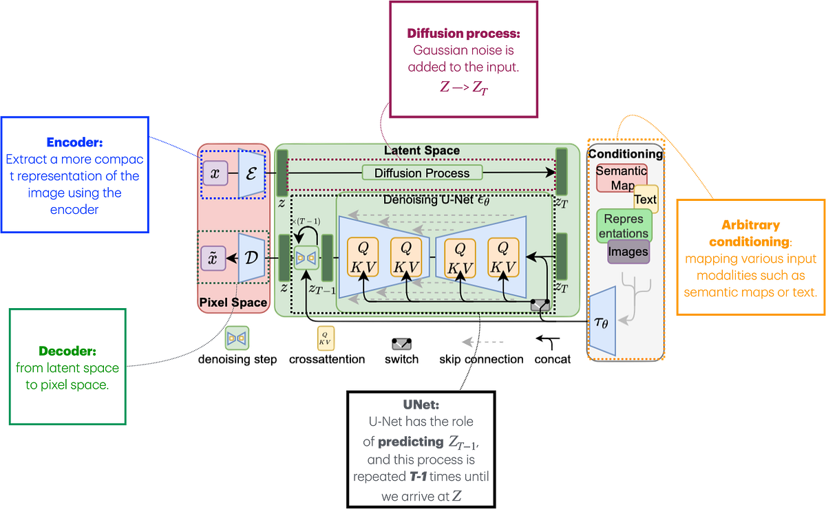
Modified from the original LDM architecture diagram by Rombach et al. (2022). Additional annotations added by an unknown author.

This is the core idea of the Latent Diffusion Model (LDM): the image formation process is decomposed into two phases:

Stage 1: Perceptual Compression is done first. This stage removes the fine, noisy, imperceptible details.

Stage 2: Generative Modeling happens next. This powerful Diffusion Model focuses entirely on the semantic and conceptual composition of the data in the small latent space.

This method reduces the computational demands for both training and sampling (creating images).

Stage 3: Building the Latent Realm (Perceptual Compression)

The first stage involves training a special tool called an Autoencoder only once. This Autoencoder has two parts: an Encoder (**E) that compresses the raw image x into a latent code z=E(x), and a Decoder (D)** that reconstructs the image x̃ from that latent code.

This compression is designed to be perceptually equivalent to the original image. It uses a combination of a perceptual loss and a patch-based adversarial objective. This blend ensures that the reconstructed images are not blurry and look locally realistic, confined to the image manifold.

A key design choice here is the compression amount, defined by the **downsampling factor, **f. This factor determines how much smaller the compressed representation is compared to the original image in terms of height (H) and width (W). It is defined as f=H/h=W/w.

For example:

• If an original image is 16×16 pixels, and the compression factor f=4 is chosen, the Encoder shrinks the image dimensions by 4 (e.g., 16÷4=4). The compressed latent code (**z)* would then be 4×4 in size (plus the channel dimension, c*).
• If the authors chose f=8, the latent code would be even smaller, 2×2 pixels.

The authors chose mild compression rates (such as f=4 or f=8). Mild compression is better because the Diffusion Model (which uses a UNet architecture that is very good at handling spatial data) does not have to rely on extreme size reduction, which would otherwise cause too much information loss and “limit the overall sample quality”. Mild factors like f=4 and f=8 find a “near-optimal point between complexity reduction and detail preservation”.

Stage 4: The Denoising Engine (Latent Diffusion)

Once the efficient latent space is ready, the main LDM (a time-conditional UNet) is trained to perform the sequential denoising task entirely in this lower-dimensional space.

This significantly increases efficiency. Because the model is working on the compressed data, it can “focus on the important, semantic bits of the data” and train in a “computationally much more efficient space”.

The training goal for this part is summarized by the LDM training objective, which is a simplified version of the reweighted variational lower bound:

Explanation: The model trains by making its guess of the True Noise (ϵ) as close as possible to the actual noise that was added to the compressed image z_t​ at time step t. Because this calculation happens in the smaller latent space z = E(x), the entire training process is dramatically faster than working on raw pixels.

This efficiency translated to results: LDMs achieved a significant FID gap of 38 compared to pixel-based DMs after the same training steps. FID (Fréchet Inception Distance) is a commonly used metric of image quality, where a lower score indicates better results. LDMs also achieved a speed-up of at least 2.7 times in sampling throughput compared to pixel-based conditional DMs for tasks like inpainting.

Till now, LDM has given good results in generating the exact image that was given as an input. But what if we want to generate a new image from text?

From onwards, we are going to discuss how to add text and generate our desired images. In this paper, external input is denoted as y.

Chapter 3: The Master Control

Beyond efficiency, LDMs were made flexible. They can be controlled by external inputs, or conditioning inputs (**y)**, such as text prompts, bounding boxes, or semantic maps.

This control is achieved by augmenting the UNet backbone with the cross-attention mechanism.

The conditioning input y is first processed by a domain-specific encoder (**τ_θ​)*. For text-to-image synthesis, this encoder is often a transformer using a BERT tokenizer. This encoded information (τ_θ​(y*)) is then mapped into the UNet via a cross-attention layer.

The Cross-Attention Mechanism (Explanation):

Cross-attention is a mechanism that allows a model to attend to and combine information from two different sequences. This mechanism acts like a smart search function that links the visual data(e.g, image) to the external command(e.g, text), defined by:

• When the UNet is focusing on generating a specific part of the image (the Query, **Q), it dynamically compares that visual need to all the concepts available in the text prompt (the Keys, **K).
• It then pulls out the corresponding semantic information (the **Values, **V) that is most relevant to that specific location in the latent space.

This system allows for multi-modal training. The conditional LDM objective becomes:

Explanation: The U-Net (ϵ_θ​) is now trained to predict the noise ϵ while simultaneously using the information provided by the encoded condition (τ_θ​(y)) to guide the generation of an image.

Chapter 4: Applications and Scale

LDMs achieved impressive results across various tasks:

• Unconditional Generation: On the CelebA-HQ dataset, LDMs reported a new state-of-the-art FID of 5.11.
• Text-to-Image: The guided LDM model achieved highly competitive scores on the MS-COCO dataset, proving it was “on par with the most recent diffusion and autoregressive methods despite using significantly fewer parameters”.
• Class-Conditional Synthesis: LDMs outperformed the leading diffusion model ADM-G on ImageNet (achieving FID 3.60 vs. ADM-G’s 4.59) while significantly reducing computational requirements and parameter count.
• High-Resolution Output: For tasks where the conditioning input is spatially aligned (like semantic synthesis or inpainting), the LDM can be applied in a convolutional manner during sampling. This allows the model to render “large, consistent images of ∼1024² px” (or megapixel images), even though it was trained on smaller 256² images.
• Inpainting: LDMs set a new state-of-the-art FID score of 1.50 for image inpainting.

Conclusion:

Latent Diffusion Models successfully provided a simple and efficient way to significantly improve the performance of denoising diffusion models without degrading their quality. They achieved this by cleverly partitioning the task: using an autoencoder for efficient perceptual compression and reserving the powerful generative U-Net for the compressed, semantic latent space.

This milestone democratized a technology previously confined to elite labs.

However, the authors noted some important limitations:

• Speed Trade-off: While much faster than pixel-based DMs, their sequential sampling process is still slower than that of GANs.
• Accuracy Limits: The small quality loss introduced by the perceptual compression (even in the mild f=4 autoencoding models) could become a bottleneck for tasks requiring extremely fine-grained accuracy in pixel space. The authors assume their super-resolution models (which achieve FID 2.8 for 4x upscaling) are already somewhat limited in this respect.
• Ethical Concerns: The increased accessibility makes it easier to create and share manipulated data (“deep fakes”). Furthermore, generative models tend to reproduce or exacerbate biases present in the training data.

The LDM architecture, through its intelligent use of the latent space and the flexible cross-attention mechanism, confirmed that computational problems in AI can often be solved by working smarter in a compressed space, leading to state-of-the-art results for the broader research community.

References:

• Rombach, R., Blattmann, A., Lorenz, D., Esser, P., & Ommer, B. (2022). High‑Resolution Image Synthesis with Latent Diffusion Models. arXiv preprint arXiv:2112.10752. https://arxiv.org/abs/2112.10752